ana4Stats: Statistical analysis tools

probAna - Probability maps

probAna is used to derive simple probability maps for a set of simulations for one avalanche track. These maps show for each point in space the fraction of simulations where a chosen parameter has exceeded a given threshold. For example, it is possible to compute the probability map for an avalanche with respect to a peak pressure threshold of 1kPa, but it is also possible to chose other result variables and threshold values.

A set of multiple avalanche simulations is required to generate these maps. The simulations can be generated with com1DFA using a parameter variation, different release-, entrainment- or resistance scenarios. An example run script is given by runAna4ProbAna.py: where firstly, com1DFA is used to perform avalanche simulations varying parameters set in the ana4Stats/probAnaCfg.ini file. Using these simulations, a probability map is generated. The output is a raster file (.asc or .tif) with values ranging from 0-1. 0 meaning that no simulation exceeded the threshold in this point in space. 1 on the contrary means that all simulations exceeded the threshold. Details on this function, as for example required inputs can be found in: ana4Stats.probAna. In addition, there is the option to use the run script runProbAnalysisOnly.py: to create probability maps for an existing set of simulations. These can be created using com1DFA or another computational module. For more details look at the section To run - example run scripts.

To run - via QGis Connector

Since version 1.6 it is possible to generate probability maps via the QGis connector. This is provided in the experimental folder of the QGis processing plugin via Probability run. A standard setup is used in which mu and release thickness are varied. Please note: samosAT friction is used instead of the default samosATAuto one.

The input requirements are the same as for com1DFA with one important difference: an additional ci95 attribute is needed for the release shapes. This describes the confidence interval for the release thickness, using the same units. I.e. if you are using a release thickness of 1.5m, you need to provide the ci in [m] as well, for example ci=0.3m. The release thickness is then automatically varied within the release thickness plus/minus the confidence interval.

To run - example run scripts

In runProbAnaCom1DFA.py, avalanche simulations are performed with the settings defined in the configuration file of com1DFA and in addition a parameter variation is performed according to the parameters set in ana4Stats/probAnaCfg.ini in the section PROBRUN. The parameters to be varied are set in varParList, the type of variation in variationType (options are: percent, range, rangefromci) and the value of the variation in variationValue. Then there are two sampling strategies to choose from, for performing the parameter variation: (1) a latin hypercube sample of all the parameters to be varied (provided in varParList) is generated and simulations are performed using sets of parameters drawn from this sample. Using sampling strategy (2) all the parameters set in PROBRUN are varied on at a time, i.e. simulations are performed for the standard settings of all parameters, except the one parameter to be varied, subsequently the other variations are performed. One probability map is created for all the different simulations and in case of sampling strategy (2), also one map per parameter that is varied once at a time, is created in addition. In order to run this example:

• first go to AvaFrame/avaframe

• copy avaframeCfg.ini to local_avaframeCfg.ini and set your desired avalancheDir

• copy ana4Stats/probAnaCfg.ini to ana4Stats/local_probAnaCfg.ini and optionally adjust variation settings

• run:

  pixi run python runAna4ProbAna.py
  

It is also possible to generate the probability maps for already existing simulations. The settings for the probability map can be set in ana4Stats/probAnaCfg.ini in the sections GENERAL and PLOT. The simulations need to be located in the avaName/Outputs/comMod/peakfiles directory, where comMod refers to the name of the computational module that has been used to create the simulation results. If com1DFA has been used, the full configuration information is accessible and hence also filtering is implemented. For other modules the only requirement is that simulation results have to be named in the following format: nameOfReleaseArea_uniqueSimulationIndicator_ModificationIndicator_simType_modelType_resultType.*

• uniqueSimulationIndicator: a string that is unique for each simulation (can also be a combination of parameter names and values in case of com1DFA this is the simHash)

• ModificationIndicator: C for changed or D for default model configuration

• simType: null, ent, res or entres regarding whether or not entrainment or resistance have been considered

• modelType: for example dfa (dense flow avalanche) or psa (powder snow avalanche)

• resultType: result variable, for example pft, ppr, pfv

For multi-layer modules (e.g. com8MoTPSA), an additional layer component (e.g. L1, L2) is inserted before the resultType: ..._modelType_layer_resultType.*

In order to run:

• first go to AvaFrame/avaframe

• copy avaframeCfg.ini to local_avaframeCfg.ini and set your desired avalancheDir

• copy ana4Stats/probAnaCfg.ini to ana4Stats/local_probAnaCfg.ini and optionally adjust GENERAL and PLOT settings

• for simulations generated with com1DFA run:

  pixi run python runProbAnalysisOnly.py
  

• all other models run:

  pixi run python runProbAnalysisOnly.py *pathToAvalancheDirectory* *comMod*
  

Another example on how to generate probability maps for avalanche simulations performed with com1DFA is given in runScripts.runProbAna, where for avaHockeyChannel simulations are performed with varying release thickness values ranging from 0.75 to 1.75 meters in steps of 0.05 meters. The resulting simulations are then used to generate the probability map with out3Plot.statsPlots.plotProbMap(). There is also the option to filter the simulations further - using the function in3Utils.fileHandlerUtils.getFilterDict() which generates a parameter dictionary for filtering according to the filter criteria set in the configuration file (ana4Stats/probAnaCfg.ini) of the ana4Stats.probAna function. In order to run this example:

• first go to AvaFrame/avaframe

• copy ana4Stats/probAnaCfg.ini to ana4Stats/local_probAnaCfg.ini

• uncomment 'FILTER' section in local_probAnaCfg.ini and insert filter parameters if you want to first filter simulations

• run:

  pixi run python runScripts/runProbAna.py
  

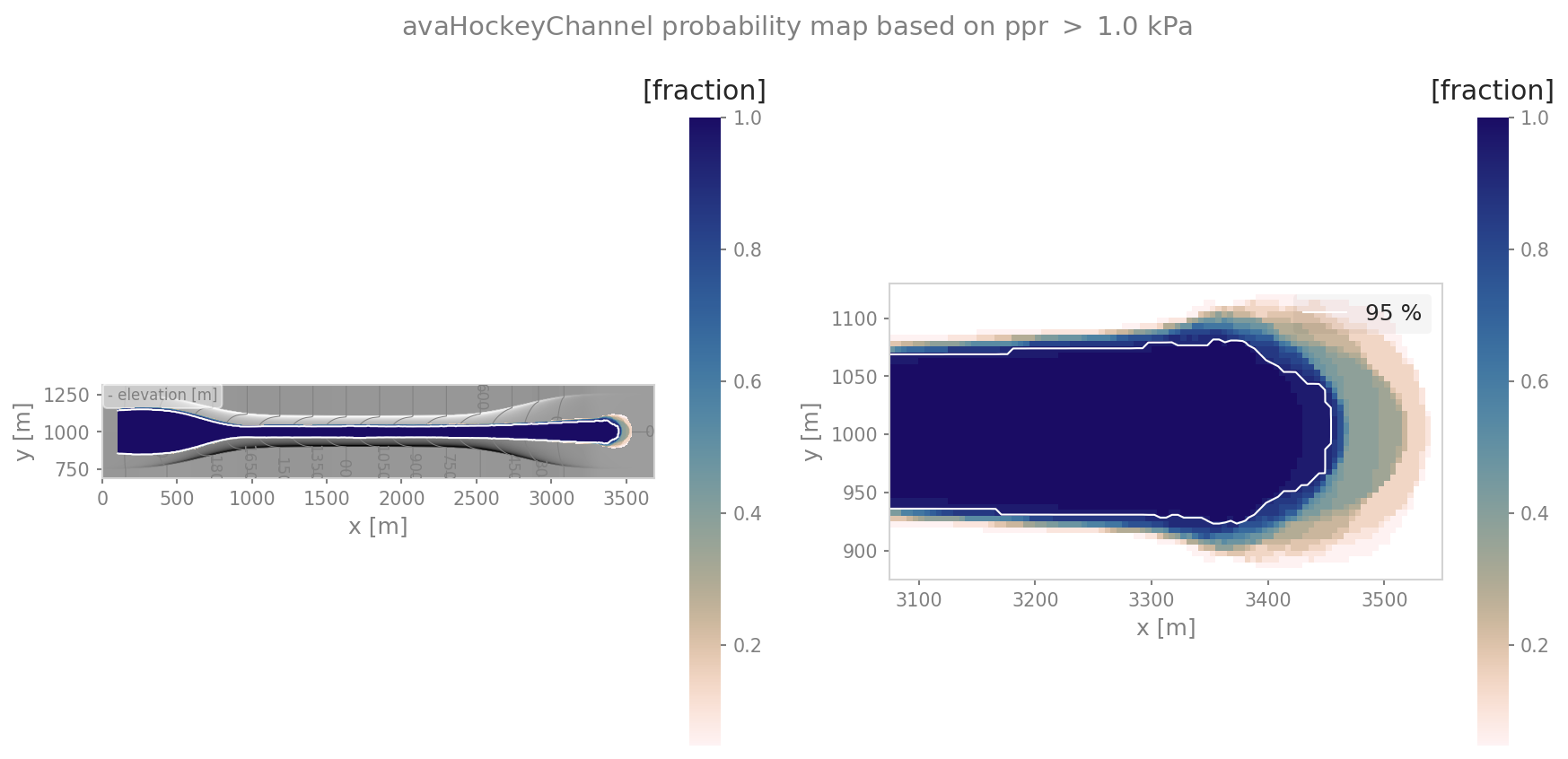
Fig. 30 Probability map example.

Theory

This point-wise probability is expressed by the relative frequency of avalanche peak flow field exceeding a certain threshold for a set of deterministic avalanche simulations derived from a range of input parameters (see [HBB19]).

getStats

In ana4Stats.getStats, functions that help to compute statistical properties of simulation results are gathered. ana4Stats.getStats.extractMaxValues() can be used to determine the maximum peak values of the simulation results. These values can then be plotted using the functions in out3Plot.statsPlots in order to visualise the statistics of a set of avalanche simulations. For further details on the specific functions, have a look at: ana4Stats.getStats.

To run

An example on how to use these statistical functions is given in runScripts.runStatsExample, where for avaHockeyChannel simulations are performed for two different release area scenarios and the release thickness is varied from 0.75 to 1.75 meters in steps of 0.05 meters. The resulting simulations are then analysed using the ana4Stats.getStats.extractMaxValues() function and plots are generated using the plotting routines from out3Plot.statsPlots . If in the configuration file ana4Stats/getStats.ini the flag aimec is set to True, additionally an ana3AIMEC: Aimec analysis is performed.

• first go to AvaFrame/avaframe

• copy ana4Stats/getStats.ini to ana4Stats/local_getStatsCfg.ini

• uncomment 'FILTER' section in ana4Stats/local_getStatsCfg.ini and insert filter parameters if you want to first filter simulations

• run:

  pixi run python runScripts/runStatsExample.py
  

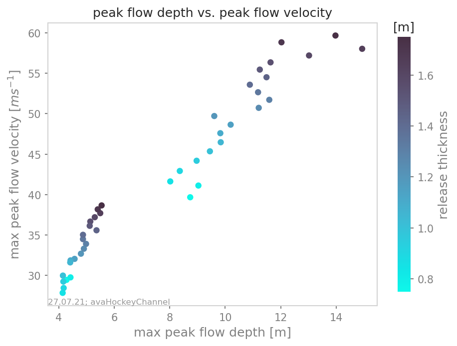
Fig. 31 Scatter plot of the hockey example with color-coded release thickness values.

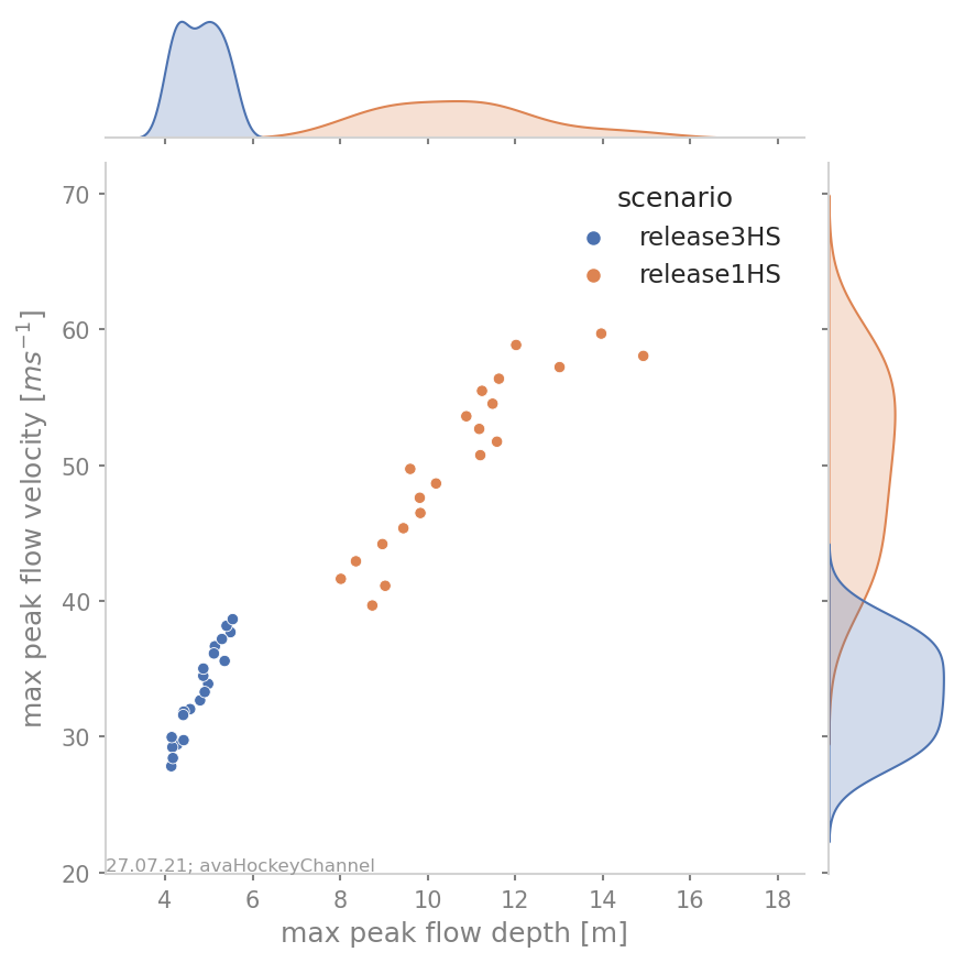
Fig. 32 Scatter plot of the hockey example including a marginal kde plot and color coded with release area scenario.