ana1Tests: Testing
In this module we gather tests with analytical or semi-analytical solution. These tests are used to evaluate the precision and accuracy of the com1DFA numerical solution.
Deviation/difference/error computation
In order to either assess the accuracy of a numerical method or to compare results it will be necessary to compute errors. The methods used to compute deviations are described in this section.
Two deviation/difference/error measures are used. The first one is based on the \(\mathcal{L}_{max}\) norm (uniform norm), the second on the Euclidean norm (\(\mathcal{L}_{2}\) norm). In both cases, the aim is to measure the deviation between a numerical solution and reference solution on an interval (one or two dimensional). Let \(f_{num}\) be the numerical solution and \(f_{ref}\) the reference solution defined on an interval \(\Omega\). The deviation is defined by \(\epsilon(x) = f_{num}(x) - f_{ref}(x)\)
Uniform norm
The \(\mathcal{L}_{max}\) norm measures the largest absolute value:
This will give an idea of the largest difference between the two solutions. It can be applied to one or two dimensional results.
It can also be normalized by dividing the uniform norm of the deviation by the uniform norm of the reference:
Euclidean norm
The \(\mathcal{L}_{2}\) norm is defined by:
This norm will give an overall measure of the deviations. It is useful to normalize the norm of the deviation either by dividing with the norm of the reference solution:
or by the measure of the interval (\(\mathcal{L}_{2}(1) = \int_{x\in \Omega}\,dx\)):
The first normalization approach will give a relative deviation in % whereas the second will give an average deviation of \(f\) on \(\Omega\).
Dambreak test
The Dambreak test compares the results of DFA simulations to the analytical solution of the “dam break” problem. In this test, a granular mass (Coulomb material) is suddenly released from rest on an inclined plane. In the case of a thickness integrated model as derived by Savage and Hutter (e.g. in [HSSN93]), an analytical solution exists. This solution is described in [FM13] and corresponds to a Riemann problem.
The problem considered has the following initial conditions:
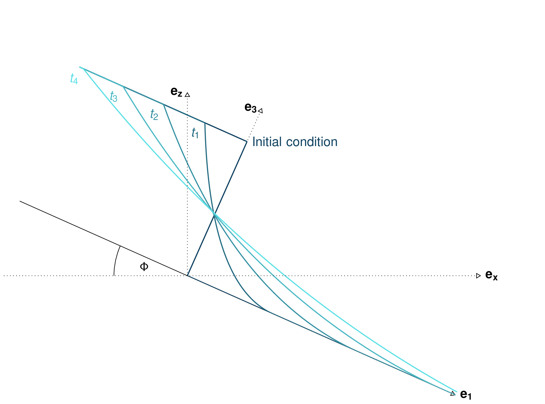
Fig. 4 Dam break theoretical evolution
The functions computing the analytical solution and comparing it to the simulation results can be
found in ana1Tests.damBreak and ana1Tests.analysisTools. Plotting routines are
located in out3Plot.outAna1Plots. The input data for this test case can be found in data/avaDamBreak.
This test produces a summary figure combining a comparison between the analytical solution and simulation result (cross cut along the flow direction) as well as a map view and an error measure plot as shown in Fig. 5.
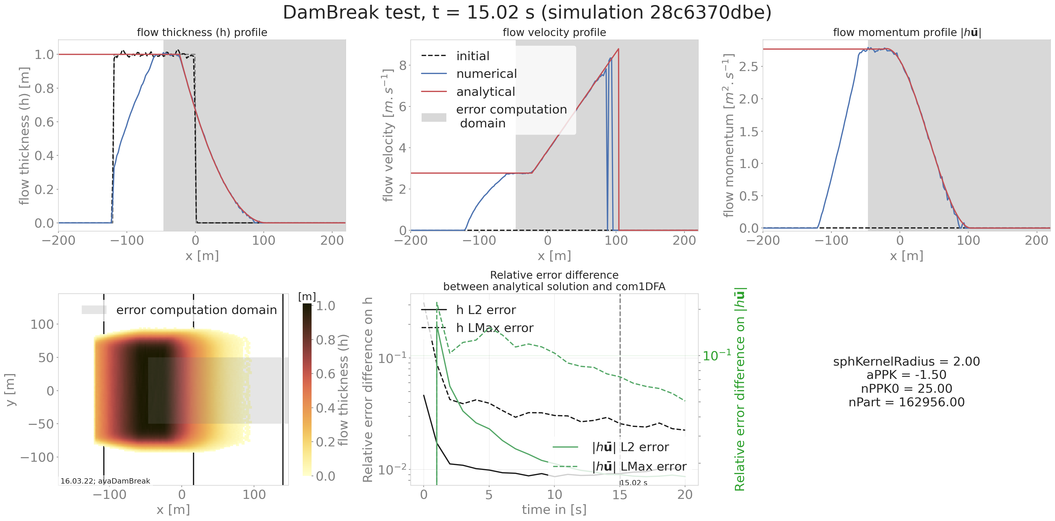
Fig. 5 Summary figure produced by the damBreak test (here for a cell size of 2m)
Another optional result is the comparison cross cut figure for all saved time steps as shown in the following animated figure.
Fig. 6 Time evolution of the flow thickness, velocity and momentum
To run
An example on how to apply this test is provided in runScripts/runDamBreak and
runScripts/runAnalyzeDamBreak.
The required input files are located in data/avaDamBreak (including the configuration file
data/avaDamBreak/Inputs/damBreak_com1DFACfg.ini). In this configuration file, there is a
specific section 'DAMBREAK' providing the required input parameters to compute the
analytical solution. In order to run the test example:
in
AvaFrame/avaframerun:pixi run python runScripts/runDamBreak.py pixi run python runScripts/runAnalyzeDamBreak.py
Similarity solution
The similarity solution is one of the few cases where a semi-analytic solution can be derived for solving the thickness integrated equations. It is a useful test case for validating simulation results coming from the dense flow avalanche computational module. This semi-analytic solution can be derived under very strict conditions and making one major assumption on the shape of the solution (symmetry/anti-symmetry of the solution around the x and y axis). The full development of the conditions and assumptions as well as the derivation of the solution is presented in details in [HSSN93]. The term semi-analytic is here used because the method enables to transform the PDE (partial differential equation) of the problem into an ODE using a similarity analysis method. Solving the ODE still requires a numerical integration but this last one is more accurate (when conducted properly) and requires less computation power than solving the PDE.
In this problem, we consider an avalanche governed by a dry friction law (Coulomb friction) flowing down an inclined plane. The released mass is initially distributed in an ellipse with a parabolic depth shape. This mass is suddenly released at \(t=0\) and flows down the inclined plane.
The ana1Tests.simiSol module provides functions to compute the semi-analytic solution and
to compare it to the output from the DFA computational module as well as some plotting routines
to visualize this solution in out3Plot.outAna1Plots.
Comparing the results from the DFA module to the similarity solution leads to the following plots:
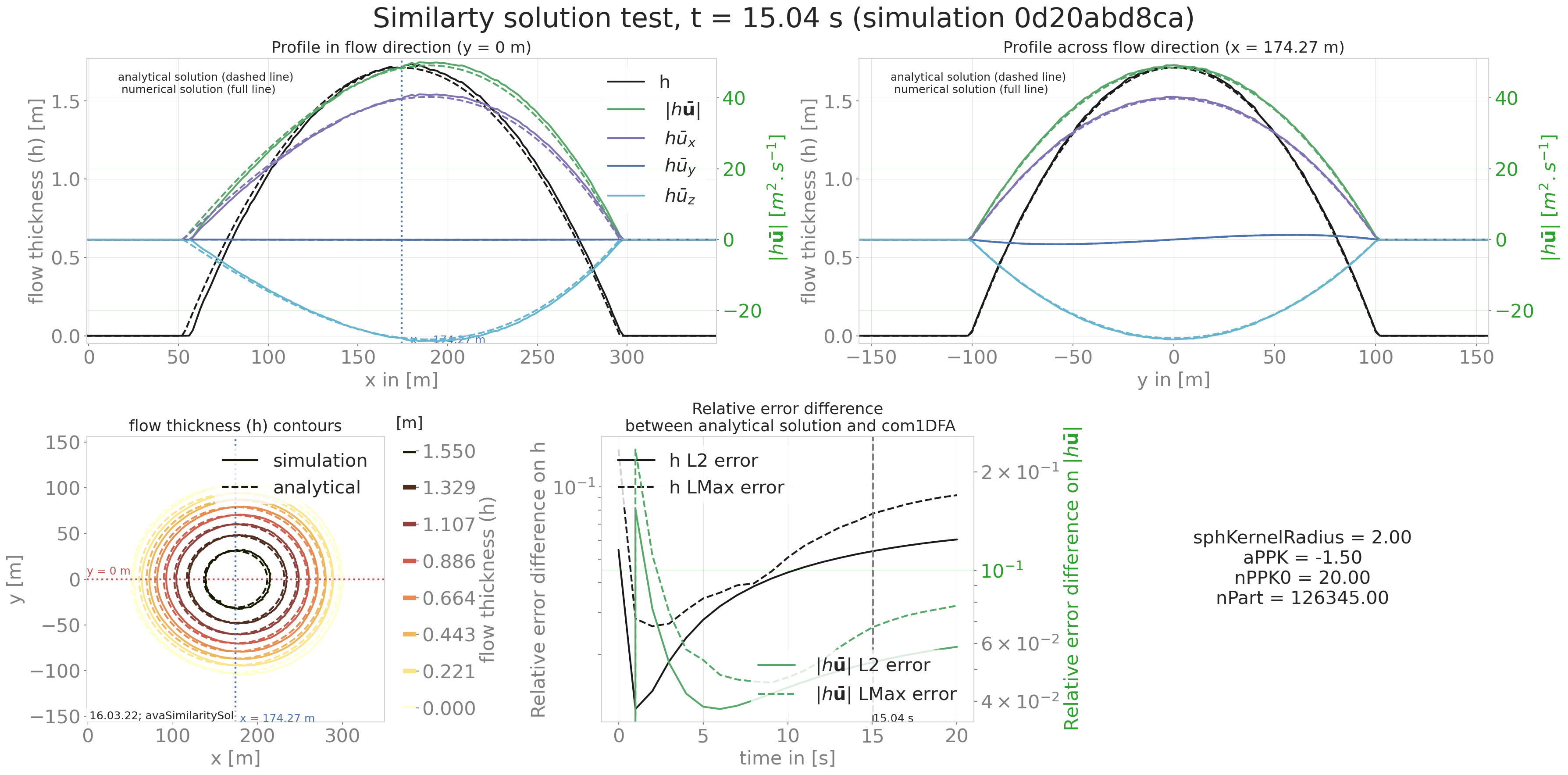
Fig. 7 Summary figure produced by the simiSol test (here for a cell size of 2m)
Fig. 8 Time evolution of the flow thickness contours in the x, y domain
Fig. 9 Time evolution of the profile in and across flow direction
To run similarity solution
A workflow example is given in runScripts/runSimilaritySol, where the semi-analytical solution
is computed and avalanche simulations are performed and both results are then compared.
The input data for this example can be found in data/avaSimilaritySol with the
configuration settings of com1DFA including a section ‘SIMISOL’ (see data/avaSimilaritySol/Inputs/simiSol_com1DFACfg.ini).
The out3Plot.outAna1Plots function generate profile plots for the flow thickness and momentum
in both flow and cross flow directions. The simulation results are plotted alongside the
analytical solution for the given time step.
Energy line test
The Energy line test compares the results of the DFA simulation to a geometrical solution that is related to the total energy of the system. Solely considering Coulomb friction this solution is motivated by the first principle of energy conservation along a simplified topography. Here friction force only depends on the slope angle. The analytical runout is the intersection of the path profile with the geometrical (\(\alpha\)) line defined by the friction angle (\(\delta\)) . From the geometrical line it is also possible to extract information about the flow mass averaged velocity at any time or position along the path profile.
Theory
Applying the energy conservation law to a material block flowing down a slope with Coulomb friction and this between two infinitesimally close time steps reads:
where \(\delta E_{fric}\) is the energy dissipation due to friction, \(\mathbf{N}\) represents the normal (to the slope surface) component of the gravity force, \(\mathbf{n}\) the normal vector to the slope surface and \(\mathbf{dl}\) is the vector representing the distanced traveled by the material between \(t\) and \(t+dt\). The normal vector reads \(\mathbf{e_z}.\mathbf{n} = cos(\theta)\), where \(\theta\) is the slope angle. \(m\) represents the mass of the material, \(g\) the gravity, \(\mu = \tan{\delta}\) the friction coefficient and friction angle, \(z\), respectively \(v\) the elevation respectively velocity of the material block. Finally, in the 2D case, \(dl = \frac{ds}{cos(\theta)}\), which means that the material is flowing in the steepest slope direction (\(\mathbf{ds}\) is the horizontal component of \(\mathbf{dl}\)).
Integrating the energy conservation between the start and a time t reads:
Speaking in terms of altitude, the energy conservation equation can be rewritten:
This result is illustrated in the following figure.
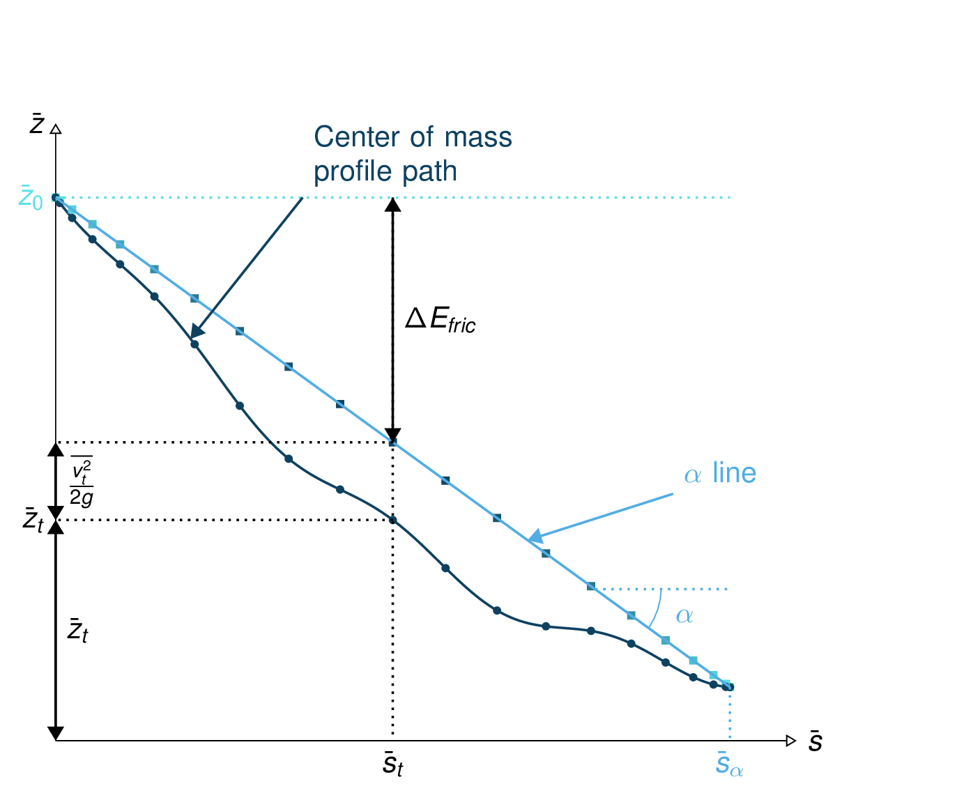
Fig. 10 Center of mass profile (dark blue line with the dots) with on top, the energy line (light blue) and the velocity altitude points (colored squared)
Considering a system of material blocks flowing down a slope with to Coulomb friction: we can sum the previous equation Eq.1 of each block after weighting it by the block mass. This leads to the mass average energy conservation equation:
where the mass average \(\bar{a}\) value of a quantity \(a\) is:
This means that the mass averaged quantities also follow the same energy conservation law when expressed in terms of altitude. The same figure as in Fig. 10 can be drawn for the center of mass profile path.
The aim is to take advantage of this energy conservation line to evaluate the DFA simulation. Computing the mass averaged path profile for the particles in the simulation and comparing it to the \(\alpha\) line allows to compute the error compared to the energy line runout. This also applies to the error on the velocity altitude. The following figures illustrate the concept.
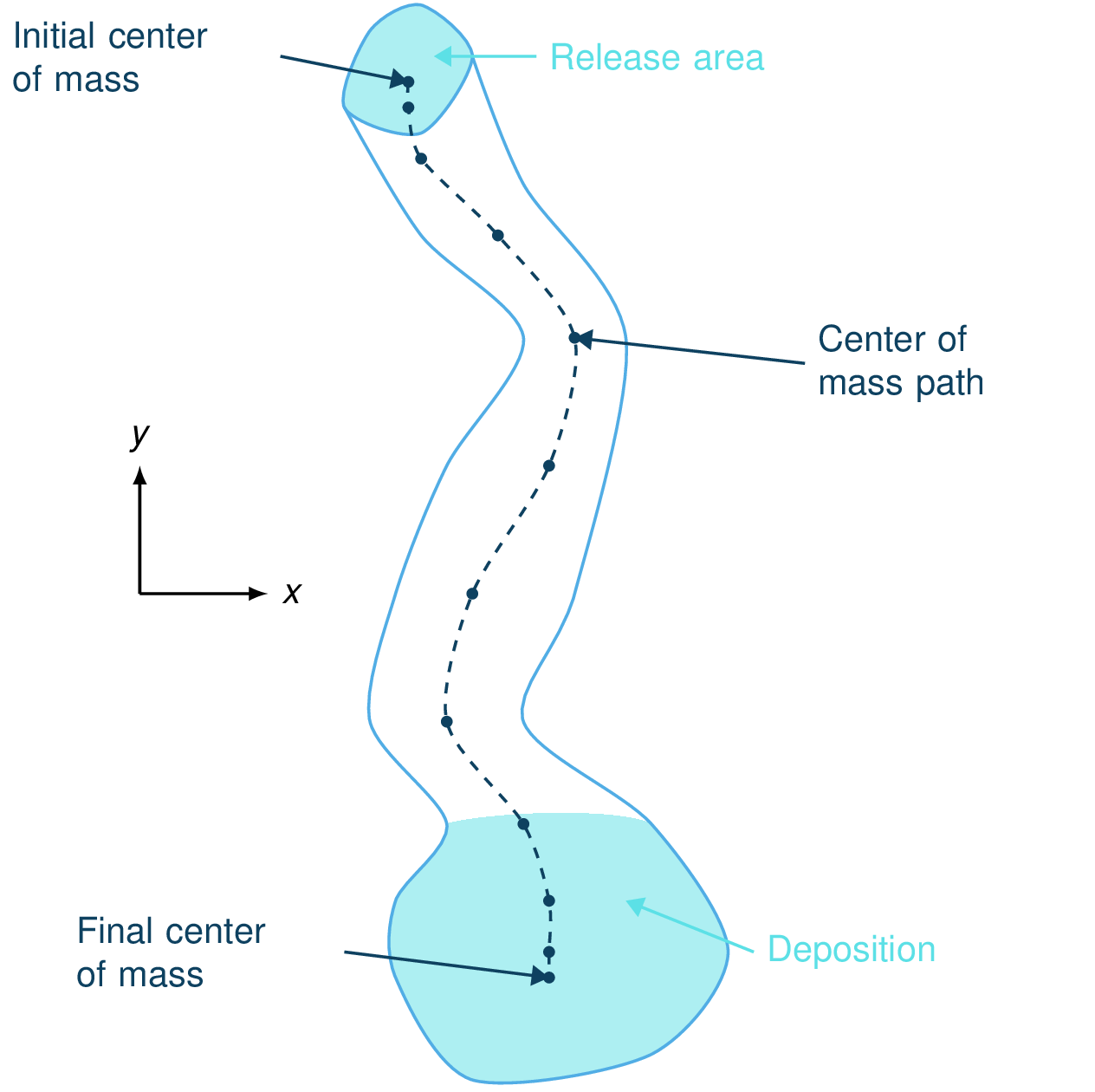
Fig. 11 View of the avalanche simulation and extracted path |
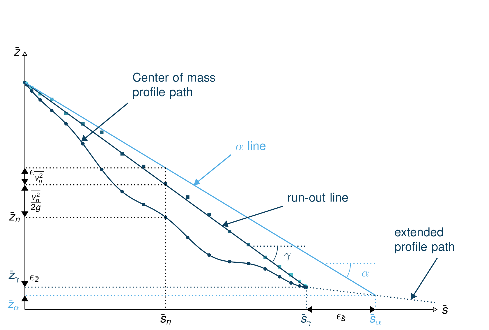
Fig. 12 Simulation path profile (dark blue curve and dots) with the runout line (dark blue line and velocity altitude squares), \(\alpha\) line and energy points |
From the different mass averaged simulation quantities and the theoretical \(\alpha\) line it is possible to extract four error indicators. The first three related to the runout point defined by the intersection between the \(\alpha\) line and the mass averaged path profile (or its extrapolation if the profile is too short) and the last one is related to the velocity :
The horizontal distance between the runout point and the end of the path profile defines the \(\epsilon_s=\bar{s}_{\gamma}-\bar{s}_{\alpha}\) error in meters.
The vertical distance between the runout point and the end of the path profile defines the \(\epsilon_z=\bar{z}_{\gamma}-\bar{z}_{\alpha}\) error in meters.
The angle difference between the \(\alpha\) line angle and the DFA simulation runout line defines the \(\epsilon_{\alpha}=\gamma-\alpha\) angle error.
The Root Mean Square Error (RMSE) between the \(\alpha\) line and the DFA simulation energy points defines an error on the velocity altitude \(\frac{\overline{v^2}}{2g}\).
Limitations and remarks
It is essential to stay where the assumptions of this test hold. Indeed, one of the important hypotheses when developing the energy solution, is that the material is flowing in the steepest slope direction (i.e. where \(dl = \frac{ds}{cos(\theta)}\) theta holds). If this hypothesis fails (as illustrated in Fig. 13), then it is not possible to develop the analytic energy solution anymore. In the 3D case, the distance vector \(\mathbf{dl}\) traveled by the particles reads \(dl = \frac{ds}{cos(\gamma)}\), where \(\gamma\) is the angle between the \(\mathbf{dl}\) vector and the horizontal plane which can differ from the slope angle \(\theta\). In this case, the energy solution is not the solution of the problem anymore and can not be used as reference.
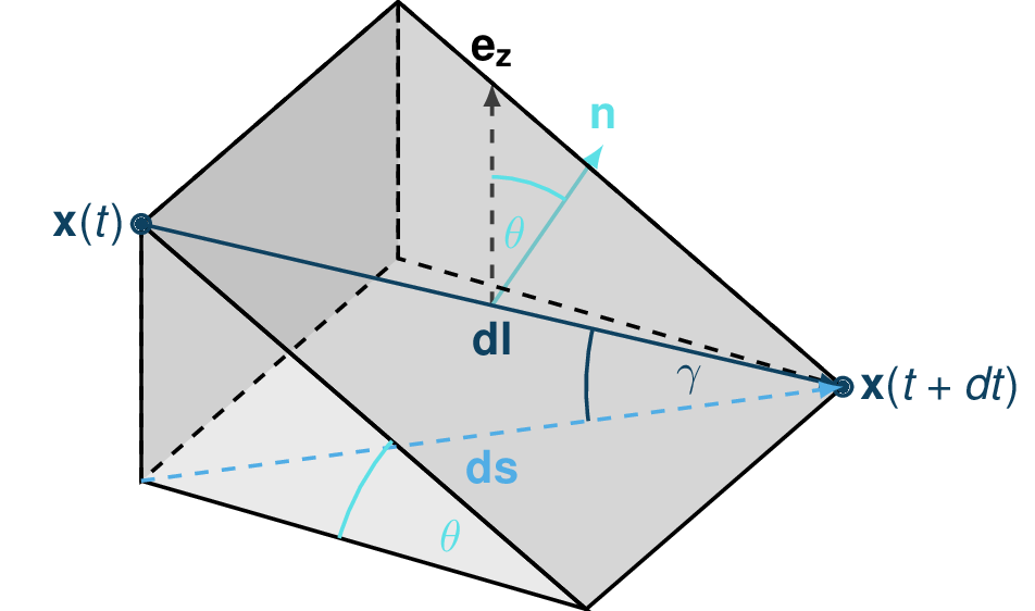
Fig. 13 Example of trajectory where the steepest descent path hypothesis fails. The mass point is traveling from \(\mathbf{x}(t)\) to \(\mathbf{x}(t+dt)\). The slope angle \(\theta\) and travel angle \(\gamma\) are also illustrated. Here \((\mathbf{e_z}.\mathbf{n}) dl = cos\theta \frac{ds}{cos\gamma} \neq ds\).
It is also possible with this test to observe the effect of terms such as curvature acceleration, artificial viscosity or pressure gradients. The curvature acceleration modifies the friction term (depending on topography curvature and particle velocity). This leads to a mismatch between the energy solution and the DFA simulation. Artificial viscosity can lead to viscous dissipation leading to shorter runouts then what the energy solution predicts. Finally, the effect of the pressure force can be studied, especially the effect of the computation options. The results of this test can also be reused for other purposes or in other test such as in the rotation test described below (Rotation test)
Procedure
First, the DFA simulation is ran (in our case using the com1DFA module) on the desired avalanche, saving the particles (at least the initial and final particles information). Then, the particles mass averaged quantities are computed (\(\bar{x}, \bar{y}, \bar{z}, \bar{s}, \bar{v^2}\)) to extract a path and path profile. Finally, the mass averaged path profile, the corresponding runout line and the expected \(\alpha\) are displayed and the runout angle and distance errors as well as the velocity altitude error are computed.
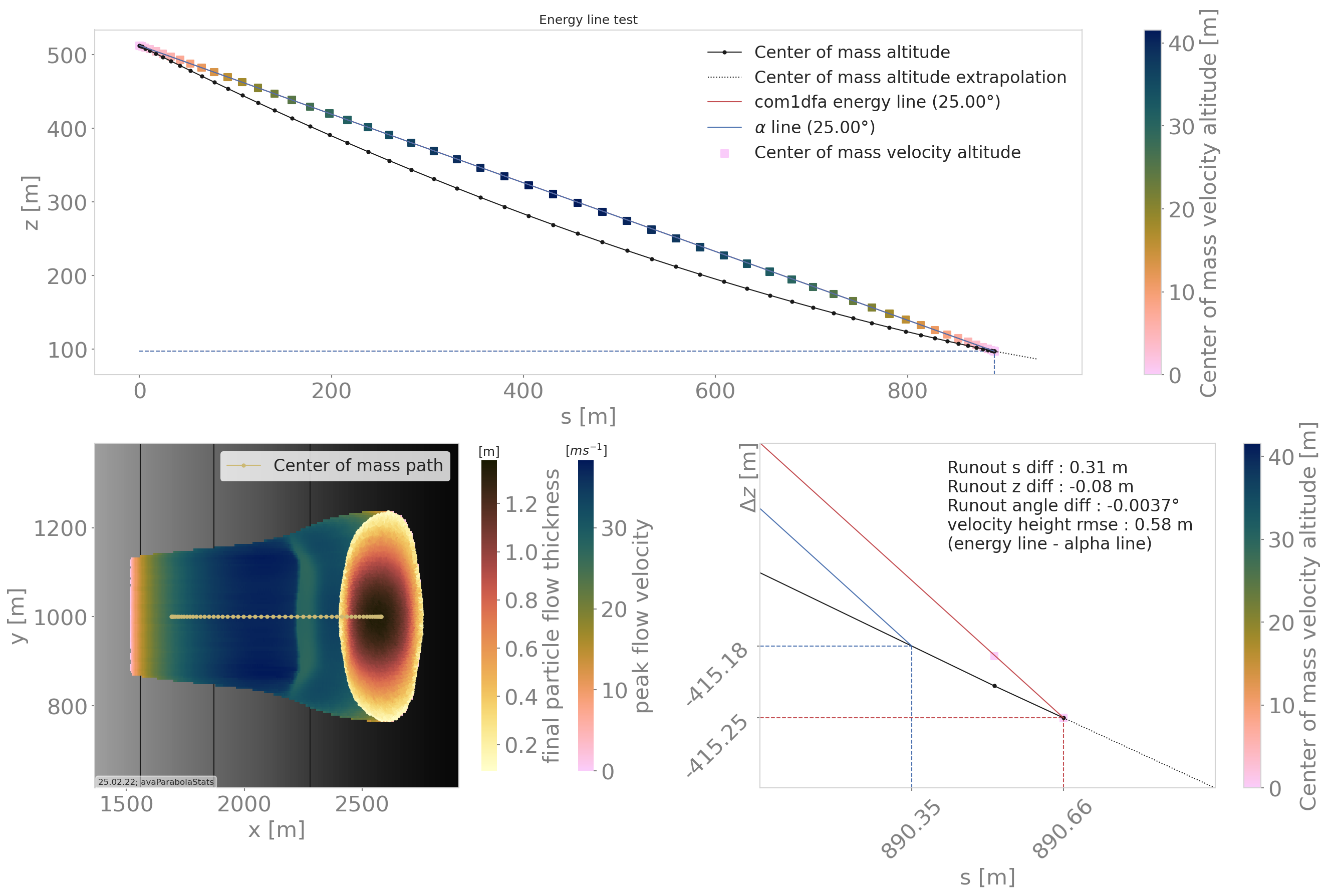
Fig. 14 Results from the ana1EnergyLineTest for the avaParabola
To run energy line test
A workflow example is given in runScripts.runEnergyLineTest.py.
Rotation test
The rotation test aims at verifying that a DFA computation module produces similar results, if not identical, independently of the underlying mesh or grid orientation used for the computation. Indeed, numerical solvers using any sort of mesh based discretization or interpolation method tend to give different results for the same physical problem, boundary conditions and initial conditions if the mesh or grid orientation is different. In this test, the same physical problem is fed to the DFA module changing only the grid orientation. The energy line test is applied to each of the simulations and the runouts are compared. An AIMEC analysis of the peak results (previously rotated so that the results are aligned) is also carried out to give a more detailed idea of the spatial differences between the simulations.
Inputs
This module requires an avalanche directory with inputs for the com1DFA and AIMEC module.
com1DFA inputs
The DEM needs to have a center of symmetry located at the origin (0, 0).
There needs to be multiple release features also symmetric in regard of the origin. These features need to be named relXXX.shp, where XXX is the rotation angle in the clockwise direction compared to the \([-\infty, 0]\) x axis.
There can also be some entrainment or resistance features (also satisfying the symmetry criterion).
ana3AIMEC inputs
The line describing the avalanche path for the reference simulation
A split point.
The most simple example is a bowl centered on (0, 0) with some circular release features all located at the same distance from the origin and a ring shaped entrainment feature (as shown on Fig. 15).
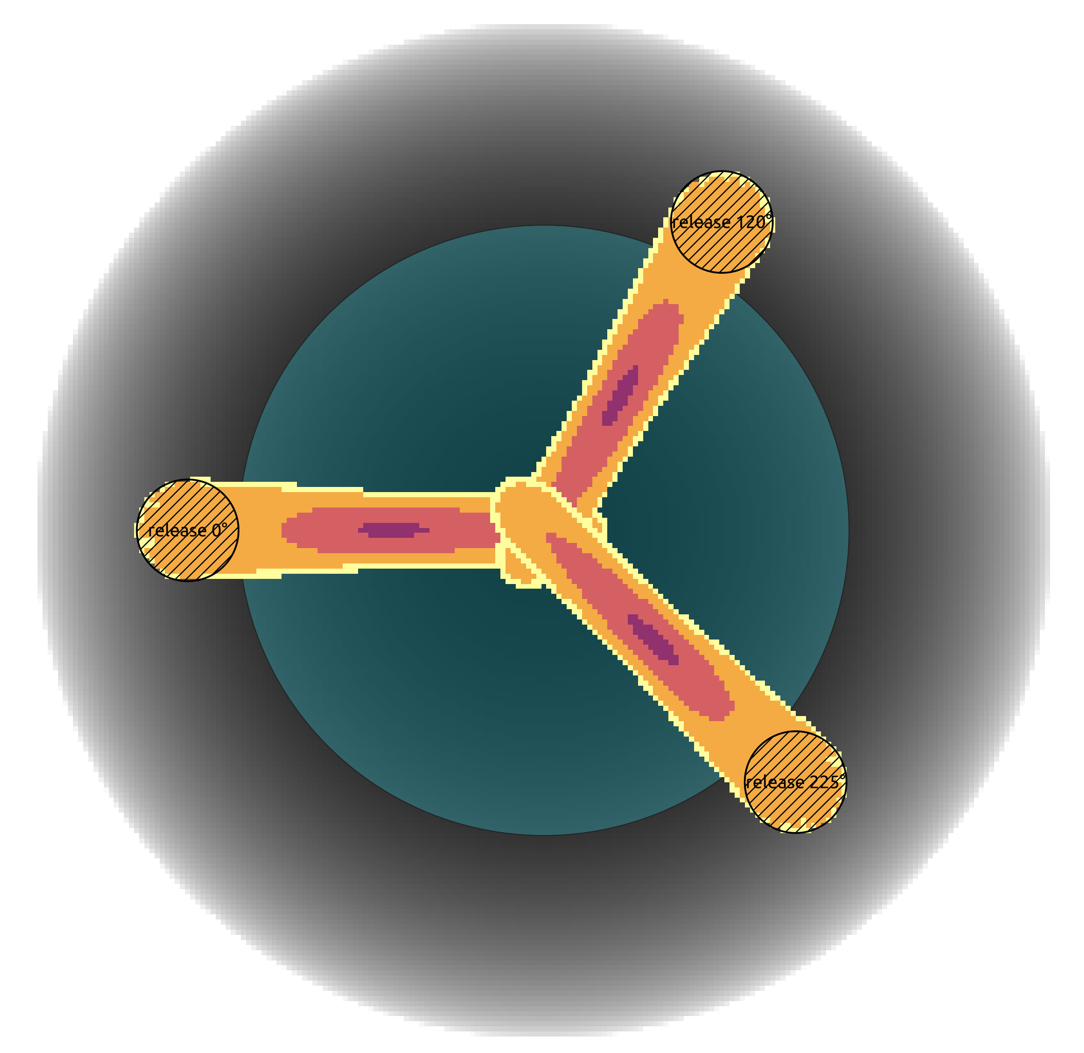
Fig. 15 Example of input data used for the rotation test and peak flow thickness result produced by the com1DFA module. In the background the bowl DEM is shown, in dashed areas (small circles) the three release features and in blue (big circle) the entrainment feature. One release feature is aligned with the x axis (rel0), the other is rotated 120° clockwise (rel120) and the last on 225° clockwise (rel225). All three input scenarios are identical (identical in terms of extend and release mass).
One then needs to specify the the com1DFA configuration (through the com1DFACfg.ini and its local version)
as well as the AIMEC configuration (through the ana3AIMECCfg.ini and its local version) and
the path generation configuration (through the pathGenerationCfg.ini and its local version).
To run rotation test
A workflow example is given in runScripts.runRotationTest.py.
Some example input data is given in avaTripleBowl (bowl topography).