com1DFA DFA-Kernel theory

Governing Equations for the Dense Flow Avalanche

The governing equations of the dense flow avalanche are derived from the incompressible mass and momentum balance on a Lagrange control volume ([Zwi00, ZKS03]).

Mass balance

(3)\[\frac{d}{dt} \int\limits_{V(t)} \rho_0 \,\mathrm{d}V = \rho_0 \frac{dV(t)}{dt} = \oint\limits_{\partial V(t)} q^{\text{ent}} \,\mathrm{d}A + \oint\limits_{\partial V(t)} q^{\text{det}} \,\mathrm{d}A\]

Where \(q^{\text{ent}}\) represents the snow entrainment rate, \(q^{\text{det}}\) the snow detrainment rate (\(q^{\text{det}} < 0\)).

Momentum balance

(4)\[\rho_0 \frac{d}{dt} \int\limits_{V(t)} u_i \,\mathrm{d}V = \oint\limits_{\partial V(t)} \sigma^{\text{tot}}_{ij}n_j \,\mathrm{d}A + \rho_0 \int\limits_{V(t)} g_i \,\mathrm{d}V, \quad i=(1,2,3)\]

We introduce the volume average of a quantity \(P(\mathbf{x},t)\):

\[\overline{P}(\mathbf{x},t) = \frac{1}{V(t)} \int\limits_{V(t)} P(\mathbf{x},t) \,\mathrm{d}V\]

and split the area integral into :

\[\oint\limits_{\partial V(t)} \sigma^{\text{tot}}_{ij}n_j \,\mathrm{d}A = \oint\limits_{\partial V(t)} \sigma_{ij}n_j \,\mathrm{d}A + F_i^{\text{ent}} + F_i^{\text{res}}, \quad i=(1,2,3)\]

\(F_i^{\text{ent}}\) represents the force required to break the entrained snow from the ground (the dense-flow bulk density is usually larger than the density of the entrained snow, i.e. \(\rho_{\text{ent}}<\rho\)) and \(F_i^{\text{res}}\) represents the resistance force due to obstacles (for example trees). This leads to in Eq.4:

\[\rho_0 \frac{dV(t) \overline{u}_i}{dt} = \rho_0 V \frac{d\overline{u}_i}{dt} + \rho_0 \overline{u}_i \frac{dV}{dt} = \oint\limits_{\partial V(t)} \sigma_{ij}n_j \,\mathrm{d}A + \rho_0 V g_i + F_i^{\text{ent}} + F_i^{\text{res}}, \quad i=(1,2,3)\]

Using the mass balance equation Eq.3, we get:

(5)\[ \begin{align}\begin{aligned}\rho_0 V \frac{d\overline{u}_i}{dt} = \oint\limits_{\partial V(t)} \sigma_{ij}n_j \,\mathrm{d}A + \rho_0 V g_i + F_i^{\text{ent}} + F_i^{\text{res}} - \overline{u}_i \oint\limits_{\partial V(t)} q^{\text{ent}} \,\mathrm{d}A - \overline{u}_i \oint\limits_{\partial V(t)} q^{\text{det}} \,\mathrm{d}A,\\\quad i=(1,2,3)\end{aligned}\end{align} \]

Boundary conditions

The free surface is defined by :

\[F_s(\mathbf{x},t) = z-s(x,y,t)=0\]

The bottom surface is defined by :

\[F_b(\mathbf{x}) = z-b(x,y)=0\]

The boundary conditions at the free surface and bottom of the flow read:

(6)\[\begin{split}\left\{\begin{aligned} &\frac{dF_s}{dt} = \frac{\partial F_s}{\partial t} + u_i\frac{\partial F_s}{\partial x_i} =0 \quad & \mbox{at }F_s(\mathbf{x},t) =0 \quad & \mbox{Kinematic BC (Material boundary)}\\ &\sigma_{ij}n_j = 0 \quad & \mbox{at }F_s(\mathbf{x},t) =0 \quad & \mbox{Dynamic BC (Traction free surface)}\\ &u_in_i = 0 \quad & \mbox{at }F_b(\mathbf{x},t) =0 \quad & \mbox{Kinematic BC (No detachment)}\\ &\tau^{(b)}_i = f(\sigma^{(b)},\overline{u},\overline{h},\rho_0,t,\mathbf{x})\quad & \mbox{at }F_b(\mathbf{x},t) =0\quad & \mbox{Dynamic BC (Chosen friction law)} \end{aligned} \right.\end{split}\]

\(\sigma^{(b)}_i = (\sigma_{kl}n_ln_k)n_i\) represents the normal stress at the bottom and \(\tau^{(b)}_i = \sigma_{ij}n_j - \sigma^{(b)}_i\) represents the shear stress at the bottom surface. \(f\) describes the chosen friction model and are described in Friction Model. The normals at the free surface (\(n_i^{(s)}\)) and bottom surface (\(n_i^{(b)}\)) are:

\[n_i^{(s,b)} = \frac{\partial F_{s,b}}{\partial x_i}\left(\frac{\partial F_{s,b}}{\partial x_j} \frac{\partial F_{s,b}}{\partial x_j}\right)^{-1/2}\]

Choice of the coordinate system

The previous equations will be developed in the orthonormal coordinate system \((B,\mathbf{v_1},\mathbf{v_2},\mathbf{v_3})\), further referenced as Natural Coordinate System (NCS). In this NCS, \(\mathbf{v_1}\) is aligned with the velocity vector at the bottom and \(\mathbf{v_3}\) with the normal to the slope, i.e.:

\[\mathbf{v_1} = \frac{\mathbf{u}}{\left\Vert \mathbf{u}\right\Vert},\quad \mathbf{v_2} = \mathbf{v_3}\wedge\mathbf{v_1}, \quad \mathbf{v_3} = \mathbf{n^{(b)}}\]

The origin \(B\) of the NCS is attached to the slope. This choice leads to:

\[n^{(b)}_i = \delta_{i3}, \quad \left.\frac{\partial b}{\partial x_i}\right\rvert_{\mathbf{0}} = 0\quad \mbox{for} \quad i=(1,2),\quad \mbox{and} \quad u^{(b)}_2 = u^{(b)}_3 = 0\]

Thickness averaged equations

In this NCS and considering a prism-like Control volume, the volume content \(V(t) = A_b(t)\overline{h}\) is obtained by multiplication of the basal area of the prism, \(A_b\), with the averaged value of the flow thickness,

(7)\[\overline{h} = \frac{1}{A_b(t)}\int\limits_{A_b(t)} [s(\mathbf{x})-b(\mathbf{x})]\,\mathrm{d}A = \frac{1}{A_b(t)}\int\limits_{A_b(t)} h(\mathbf{x})\,\mathrm{d}A,\qquad \overline{u}_i = \frac{1}{V(t)}\int\limits_{V(t)} u_i(\mathbf{x})\,\mathrm{d}V\]

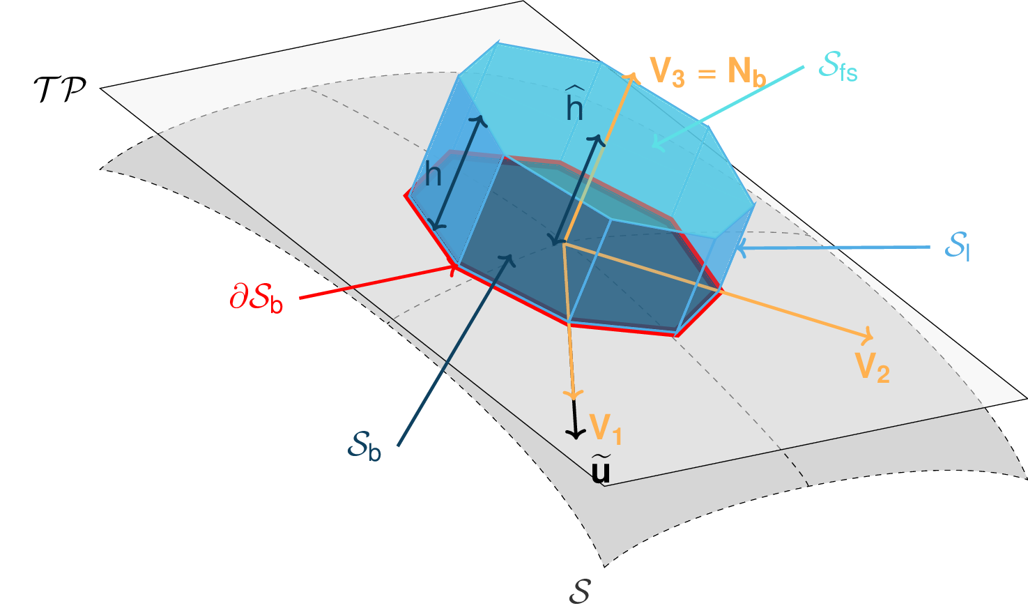
Fig. 43 Small Lagrangian prism-like Control volume

Entrainment

The Snow entrainment processes are plowing at the front of the avalanche and erosion at the bottom. Please note: com1DFA uses one or the other process, not both at the same time (default: erosion). The other process is set to zero. The entrainment rate at the front \(\dot{q}^{\text{plo}}\) can be expressed as a function of the properties of the entrained snow (density \(\rho_{\text{ent}}\) and snow thickness \(h_{\text{ent}}\)), the velocity of the avalanche at the front \(\overline{\mathbf{u}}\) and length \(w_f\) of the front (measured perpendicularly to the flow velocity \(\overline{\mathbf{u}}\)). It obviously only happens on the front of the avalanche:

(8)\[\oint\limits_{\partial V(t)} \dot{q}^{\text{plo}}\,\mathrm{d}A = \int\limits_{l_{\text{front}}}\int_b^s \dot{q}^{\text{plo}}\, \mathrm{d}{l}\,\mathrm{d}{z} = \rho_{\text{ent}}\,w_f\,h_{\text{ent}}\,\left\Vert \overline{\mathbf{u}}\right\Vert\]

The entrainment rate at the bottom \(\dot{q}^{\text{ero}}\) can be expressed as a function of the bottom area \(A_b\) of the control volume, the velocity of the avalanche \(\overline{\mathbf{u}}\), the bottom shear stress \(\tau^{(b)}\) and the specific erosion energy \(e_b\):

(9)\[\oint\limits_{\partial V(t)} \dot{q}^{\text{ero}}\,\mathrm{d}A = \int\limits_{A_b} \dot{q}^{\text{ero}}\, \mathrm{d}A = A_b\,\frac{\tau^{(b)}}{e_b}\,\left\Vert \overline{\mathbf{u}}\right\Vert\]

This leads in the mass balance Eq.3 to :

(10)\[\frac{\mathrm{d}V(t)}{\mathrm{d}t} = \frac{\mathrm{d}(A_b\overline{h})}{\mathrm{d}t} = \frac{\rho_{\text{ent}}}{\rho_0}\,w_f\,h_{\text{ent}}\,\left\Vert \overline{\mathbf{u}}\right\Vert + \frac{A_b}{\rho_0}\,\frac{\tau^{(b)}}{e_b}\,\left\Vert \overline{\mathbf{u}}\right\Vert\]

The force \(F_i^{\text{ent}}\) required to break the entrained snow from the ground is expressed as a function of the required breaking energy per fracture surface unit \(e_s\) (\(J.m^{-2}\)), the deformation energy per entrained mass element \(e_d\) (\(J.kg^{-1}\)) and the entrained snow thickness ([FKF+15, SFF+08, Sam07]):

(11)\[F_i^{\text{ent}} = -w_f\,(e_s+\,q^{\text{ent}}\,e_d),\]

where \(q^{\text{ent}}\) refers to the entrainable mass per surface area (\(kg.m^{-2}\)) defined by \(q^{\text{ent}}: =\rho^{\text{ent}} h^{\text{ent}}\) which depending on whether entrainment is due to ploughing or erosion, is derived using the integral of \(\dot{q}^{\text{plo}}\), or respectively \(\dot{q}^{\text{ero}}\), over time.

Detrainment

The detrained snow \(M_{det}\) at obstacles (e.g., trees) is computed by following the approach of ([FBT+14]):

(12)\[\oint\limits_{\partial V(t)} \dot{q}^{\text{det}}\,\mathrm{d}A = \frac{\mathrm{d}M_{det}(t)}{\mathrm{d}t} = - K\,\frac{A_b}{\left\Vert \overline{\mathbf{u}}\right\Vert}\]

The parameter \(K\) (\(Pa\)) depends on the structure of the obstacles and the properties of the snow.

Currently, detrainment is only applicable when using the ResistanceModel =  default. In this case, if flow thickness or flow velocity fall below minimum thresholds defined in the configuration file, detrainment is applied.

Resistance

The force \(F_i^{\text{res}}\) due to obstacles is expressed as a function of the characteristic coefficient \(c_{\text{resH}}\):

\[F_i^{\text{res}} = -c_{\text{res}H}\,\rho_0\,A\, \overline{u}^2\, \frac{\overline{u}_i}{\|\overline{u}\|}\]

Note

In versions earlier than 1.13, this formula included information about tree diameter, tree spacing, etc. and was dependent on an effective thickness (a function of flow thickness). Please check out previous documentation versions for details.

In the default setup (ResistanceModel =  default and detrainment = True) either detrainment or increased friction (using \(F_i^{\text{res}}\)) is applied, depending on the flow thickness (FT) and velocity (FV) at the current cell and time step:

• FV OR FT below min thresholds: apply only detrainment, no increased friction

• FV AND FT within min and max thresholds: no detrainment, only apply increased friction

• FV OR FT above max thresholds: no detrainment and no increased friction applied

If detrainment = False, the additional resistance force is accounted for in the entire resistance area.

Adaptive surface

When the flowing mass changes (due to detrainment, entrainment and/or stopping = velocity is zero), the surface topography can be adapted (if adaptSfcDetrainment = 1, adaptSfcEntrainment = 1 and/or adaptSfcStopped = 1, respectively).

The detrained/ entrained/ stopped mass is converted into the corresponding snow depth changes \(h_{det}, h_{ent}, h_{stop}\) at the location of the particle using the Particles to mesh method.

The adapted surface at a specific time step \(z(t)\) is computed as (with \(h_{det}, h_{ent}, h_{stop} > 0\)):

\[z(t) = z(t=0) + \sum_{i=0}^t (h_{det}(i) + h_{stop}(i) - h_{ent}(i))\]

In every time step the surface is adapted, the Cell normals and Cell area are also adapted.

If the surface is adapted due to stopped particles (velocity = 0 and adaptSfcStopped = 1), the stopped particles are deleted and stored in a separate dictionary stoppedParticles (see Particle properties).

Note

This feature requires more detailed testing and may cause numerical problems if the change in snow depth is very high.

Surface integral forces

The surface integral is split in three terms, an integral over \(A_b\) the bottom \(x_3 = b(x_1,x_2)\), \(A_s\) the top \(x_3 = s(x_1,x_2,t)\) and \(A_h\) the lateral surface. Introducing the boundary conditions Eq.6 leads to:

\[\begin{split}\begin{aligned} \oint\limits_{\partial{V(t)}}\sigma_{ij}n_j\,\mathrm{d}A & = \int\limits_{A_b}\underbrace{\sigma_{ij}\,n_j^{(b)}}_{-\sigma_{i3}}\,\mathrm{d}A + \int\limits_{A_s}\underbrace{\sigma_{ij}\,n_j^{(s)}}_{0}\,\mathrm{d}A + \int\limits_{A_h}\sigma_{ij}\,n_j\,\mathrm{d}A\\ &= -A_b\overline{\sigma}_{i3}^{(b)} + \oint\limits_{\partial A_b}\left(\int_b^s\sigma_{ij}\,n_j\,\mathrm{d}x_3\right)\,\mathrm{d}l \end{aligned}\end{split}\]

Which simplifies the momentum balance Eq.5 to:

(13)\[\begin{split}\begin{aligned} \rho_0 V \frac{d\overline{u}_i}{dt} = & \oint\limits_{\partial A_b}\left(\int_b^s\sigma_{ij}\,n_j\, \mathrm{d}x_3\right)\,\mathrm{d}l -A_b\overline{\sigma}_{i3}^{(b)} + \rho_0 V g_i + F_i^{\text{ent}} + F_i^{\text{res}} \\ - \overline{u}_i \oint\limits_{\partial V(t)} q^{\text{ent}} \,\mathrm{d}A - \overline{u}_i \oint\limits_{\partial V(t)} q^{\text{det}} \,\mathrm{d}A, &\quad i=(1,2,3) \end{aligned}\end{split}\]

The momentum balance in direction \(x_3\) (normal to the slope) is used to obtain a relation for the vertical distribution of the stress tensor ([Sam07]). Due to the choice of coordinate system and because of the kinematic boundary condition at the bottom, the left side of Eq.13 can be expressed as a function of the velocity \(\overline{u}_1\) in direction \(x_1\) and the curvature of the terrain in this same direction \(\frac{\partial^2{b}}{\partial{x_1^2}}\) ([Zwi00]):

\[\rho\,A_b\,\overline{h}\,\frac{\,\mathrm{d}\overline{u}_3}{\,\mathrm{d}t} = \rho\,A_b\,\overline{h}\,\frac{\partial^2{b}}{\partial{x_1^2}}\,\overline{u}_1^2,\]

rearranging the terms in the momentum equation leads to:

(14)\[\overline{\sigma}_{33}(x_3) = \rho_0\,(s-x_3)\left(g_3-\frac{\partial^2{b}}{\partial{x_1^2}}\,\overline{u}_1^2\right)+ \frac{1}{A_b} \oint\limits_{\partial A_b}\left(\int_{x_3}^s\sigma_{3j}\,n_j\,\mathrm{d}x_3\right)\,\mathrm{d}l\]

Non-dimensional Equations

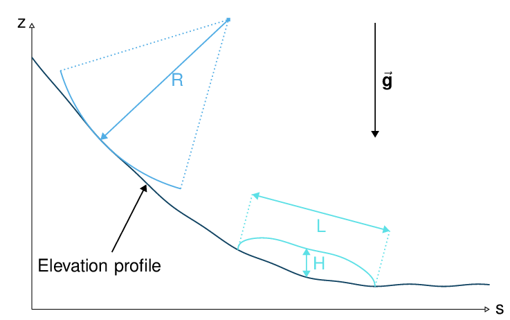
Fig. 44 Characteristic size of the avalanche along its path (from [Zwi00], modified)

The previous equations Eq.13 and Eq.14 can be further simplified by introducing a scaling based on the characteristic values of the physical quantities describing the avalanche. The characteristic length L, the thickness H, the acceleration due to gravity g and the characteristic radius of curvature of the terrain R are the chosen quantities. From those values, it is possible to form two non dimensional parameters that describe the flow:

• Aspect ratio: \(\qquad\qquad\varepsilon = H / L\qquad\)

• Curvature: \(\qquad\lambda = L / R\qquad\)

The different properties involved are then expressed in terms of characteristic quantities \(L\), \(H\), \(g\), \(\rho_0\) and \(R\) (see Fig. 44):

\[\begin{split}\begin{aligned} x_i &= L\, x_i^*\\ (dx_3,h,\overline{h}) &= H\,(dx_3^*,h^*,\overline{h}^*)\\ A_b &= L^2\, A_b^*\\ t &= \sqrt{L/\text{g}}\, t^*\\ \overline{u_i} &= \sqrt{\text{g}L}\,\overline{u_i}^*\\ \text{g}_i &= \text{g} \, \text{g}_i^*\\ \frac{\partial^2{b}}{\partial{x_1}^2} &= \frac{1}{R}\,\frac{\partial^2{b^*}}{\partial{x_1}^{*2}}\end{aligned}\end{split}\]

The normal part of the stress tensor is directly related to the hydro-static pressure:

\[\sigma_{ii} = \rho_0\,\text{g}\,H\,\sigma_{ii}^*\]

The dimensionless properties are indicated by a superscripted asterisk. Introducing those properties in Eq.14, leads to :

(15)\[\overline{\sigma^*}_{33} = \left(g^*_3-\lambda\frac{\partial^2{b^*}}{\partial{x_1^{*2}}}\,\overline{u}_1^{*2}\right) (s^*-x^*_3) + \underbrace{\varepsilon\oint\limits_{\partial A_b^*}\left(\int\limits_{x^*_3}^{s^*}\sigma^*_{31}\,\mathrm{d}x^*_3\right)\,\mathrm{d}l^*}_{O(\varepsilon)}.\]

The height, H of dense flow avalanches is assumed to be small compared to its length, L. Meaning that the equations are examined in the limit \(\varepsilon \ll 1\). It is then possible to neglect the last term in Eq.15 which leads to (after reinserting the dimensions):

(16)\[\overline{\sigma}_{33}(x_3) = \rho_0\,\underbrace{\left(g_3-\overline{u_1}^2\,\frac{\partial^2{b}}{\partial{x_1^2}}\right)}_{g_\text{eff}} \left[\overline{h}-x_3\right]\]

And at the bottom of the avalanche, with \(x_3 = 0\), the normal stress can be expressed as:

(17)\[\overline{\sigma}^{(b)}_{33} = \rho_0\,\left(g_3-\overline{u_1}^2\,\frac{\partial^2{b}}{\partial{x_1^2}}\right)\,\overline{h}\]

Calculating the surface integral in equation Eq.13 requires to express the other components of the stress tensor. Here again a magnitude consideration between the shear stresses \(\sigma_{12} = \sigma_{21}\) and \(\sigma_{13}\). The shear stresses are based on a generalized Newtonian law of materials, which controls the influence of normal stress and the rate of deformation through the viscosity.

\[\tau_{ij} = \eta\left(\frac{\partial{u_i}}{\partial{x_j}}+\frac{\partial{u_j}}{\partial{x_i}}\right), ~ i\neq j\]

Because \(\partial x_1\) and \(\partial x_2\) are of the order of \(L\), whereas \(\partial x_3\) is of the order of \(H\), it follows that:

\[O\left(\frac{\sigma_{12}}{\sigma_{13}}\right) = \frac{H}{L} = \varepsilon \ll 1\]

and thus \(\sigma_{12} = \sigma_{21}\) is negligible compared to \(\sigma_{13}\). \(\sigma_{13}\) is expressed using the bottom friction law \(\tau^{(b)}_i = f(\sigma^{(b)},\overline{u},\overline{h},\rho_0,t,\mathbf{x})\) introduced in Eq.6.

In addition, a relation linking the horizontal normal stresses, \(\sigma_{ii}\), \(i = (1,2)\), to the vertical pressure distribution given by Eq.17 is introduced. In complete analogy to the arguments used by Savage and Hutter ([SH89]) the horizontal normal stresses are given as:

\[\sigma_{ii} = K_{(i)}\,\sigma_{33}\]

Where \(K_{(i)}\) are the earth pressure coefficients (cf. [Sal04, ZKS03]):

\[\begin{split}\sigma_{11} &= K_{x~akt/pass}\,\sigma_{33}\\ \sigma_{22} &= K_{y~akt/pass}^{(x~akt/pass)}\,\sigma_{33}\end{split}\]

With the above specifications, the integral of the stresses over the flow height is simplified in equation Eq.13 to:

\[\int\limits_b^s\sigma_{ij}\,\mathrm{d}x_3 = \int\limits_b^s K_{(i)}\,\sigma_{33}\,\mathrm{d}x_3 = K_{(i)}\,\frac{\overline{h}\,\sigma^{(b)}}{2}\]

and the momentum balance can be written:

(18)\[\begin{split}\begin{aligned} \rho_0\,A\,\overline{h}\,\frac{\,\mathrm{d}\overline{u}_i}{\,\mathrm{d}t} = &\rho_0\,A\,\overline{h}\,g_i + \underbrace{K_{(i)}\,\oint\limits_{\partial{A}}\left(\frac{\overline{h}\,\sigma^{(b)}}{2}\right)n_i\,\mathrm{d}l}_{F_i^{\text{lat}}} \underbrace{-\delta_{i1}\,A\,\tau^{(b)}}_{F_i^{\text{bot}}} \underbrace{- \rho_0\,A\,h_{\text{eff}}\,C_{\text{res}}\,\overline{\mathbf{u}}^2\,\frac{\overline{u_i}}{\|\overline{\mathbf{u}}\|}}_{F_i^{\text{res}}}\\ &- \overline{u_i}\,\rho_0\,\frac{\mathrm{d}\left(A\,\overline{h}\right)}{\mathrm{d}t} + F_i^{\text{ent}} \end{aligned}\end{split}\]

with

\[C_{\text{res}} = \frac{1}{2}\,\overline{d}\,\frac{c_w}{s_{\text{res}}^2}.\]

The mass balance Eq.10 remains unchanged:

(19)\[\frac{\mathrm{d}V(t)}{\mathrm{d}t} = \frac{\mathrm{d}\left(A_b\overline{h}\right)}{\mathrm{d}t} = \frac{\rho_{\text{ent}}}{\rho_0}\,w_f\,h_{\text{ent}}\,\left\Vert \overline{\mathbf{u}}\right\Vert + \frac{A_b}{\rho_0}\,\frac{\tau^{(b)}}{e_b}\,\left\Vert \overline{\mathbf{u}}\right\Vert - \frac{K}{\rho_0}\,\frac{A_b}{\left\Vert \overline{\mathbf{u}}\right\Vert}\]

The unknown \(\overline{u}_1\), \(\overline{u}_2\) and \(\overline{h}\) satisfy Eq.17, Eq.18 and Eq.19. In equation Eq.18 the bottom shear stress \(\tau^{(b)}\) remains unknown, and and a constitutive equation has to be introduced in order to completely solve the equations.

Friction Model

The problem can be solved by introducing constitutive equations which describe the behaviour of a material due to stress. For granular materials like avalanches the basal shear stress tensor \(\tau^{(b)}\) is expressed as a function of the flow state of the avalanche (Granular friction models).

(26)\[\tau^{(b)}_i = f(\sigma^{(b)},\overline{u},\overline{h},\rho_0,t,\mathbf{x})\]

With

\[\begin{split}\begin{aligned} &\sigma^{(b)} \qquad &\text{normal component of the stress tensor}\\ &\overline{u} \qquad &\text{average velocity}\\ &\overline{h} \qquad &\text{average flow thickness}\\ &\rho_0 \qquad &\text{density}\\ &t \qquad &\text{time}\\ &\mathbf{x} \qquad &\text{position vector}\end{aligned}\end{split}\]

For solid-fluid mixtures like debris flows, where the properties of the fluid phase are dominating the flow process, the shear stress tensor is, among other things, a function of a consistency factor \(K\) and the shear rate \(\dot\gamma\) (Rheological Models).

(21)\[\tau^{(b)}_i = f(K,\dot\gamma,\overline{h},\rho_m,t,\mathbf{x})\]

With

\[\begin{split}\begin{aligned} &K \qquad &\text{consistency factor of the solid-fluid mixture}\\ &\dot\gamma \qquad &\text{shear rate}\\ &\overline{h} \qquad &\text{average flow thickness}\\ &\rho_m \qquad &\text{density of the solid-fluid mixture}\\ &t \qquad &\text{time}\\ &\mathbf{x} \qquad &\text{position vector}\end{aligned}\end{split}\]

Several friction models already implemented in the simulation tool are described in the following sections.

Granular friction models

Mohr-Coulomb friction model

The Mohr-Coulomb friction model describes the friction interaction between twos solids. The bottom shear stress simply reads:

(22)\[\tau^{(b)} = \tan{\delta}\,\sigma^{(b)}\]

\(\tan{\delta}=\mu\) is the friction coefficient (and \(\delta\) the friction angle). The bottom shear stress linearly increases with the normal stress component \(\sigma^{(b)}\) ([BSG99, Sam07, WHP04, Zwi00]).

With this friction model, an avalanche starts to flow if the slope inclination is steeper than the friction angle \(\delta\). In the case of an infinite slope of constant inclination, the avalanche velocity would increase indefinitely. This is unrealistic to model snow avalanches because it leads to over prediction of the flow velocity. The Mohr-Coulomb friction model is on the other hand well suited to model granular flow. Because of its relative simplicity, this friction model is also very convenient to derive analytic solutions and validate the numerical implementation.

Chezy friction model

The Chezy friction model describes viscous friction interaction. The bottom shear stress then reads:

(23)\[\tau^{(b)} = c_{\text{dyn}}\,\rho_0\,\bar{u}^2\]

\(c_{\text{dyn}}\) is the viscous friction coefficient. The bottom shear stress is a quadratic function of the velocity. ([BSG99, Sam07, WHP04, Zwi00]).

This model enables to reach more realistic velocities for avalanche simulations. The draw back is that the avalanche doesn’t stop flowing before the slope inclination approaches zero. This implies that the avalanche flows to the lowest local point.

Voellmy friction model

Anton Voellmy was a Swiss engineer interested in avalanche dynamics [Voe55]. He first had the idea to combine both the Mohr-Coulomb and the Chezy model by summing them up in order to take advantage of both. This leads to the following friction law:

(24)\[\tau^{(b)} = \tan{\delta}\,\sigma^{(b)} + \frac{g}{\xi}\,\rho_0\,\bar{u}^2\]

where \(\xi\) is the turbulent friction term. This model is described as Voellmy-Fluid [Sal04, Sam07].

It is also possible to use spatially variable values for the friction parameters \(\mu =f(x, y)\) and \(\xi =f(x, y)\). For this option, raster files with values for \(\mu\) and \(\xi\) need to be provided as input data covering the same extent as the digital elevation model.

VoellmyMinShear friction model

In order to increase the friction force and make the avalanche flow stop on steeper slopes than with the Voellmy friction relation, a minimum shear stress can be added to the Voellmy friction relation. This minimum value defines a shear stress under which the snowpack doesn’t move, and induces a strong flow deceleration. This expression of the basal layer friction model also resembles the one used in the swiss RAMMS model, where the Voellmy model is modified by adding a yield stress supposed to account for the snow cohesion (https://ramms.slf.ch/en/modules/debrisflow/theory/friction-parameters.html).

(25)\[\tau^{(b)} = \tau_0 + \tan{\delta}\,\sigma^{(b)} + \frac{g}{\xi}\,\rho_0\,\bar{u}^2\]

SamosAT friction model

SamosAT friction model is a modification of some more classical models such as Voellmy model Voellmy friction model. The basal shear stress tensor \(\tau^{(b)}\) is expressed as ([Sam07]):

(26)\[\tau^{(b)} = \tau_0 + \tan{\delta}\,\left(1+\frac{R_s^0}{R_s^0+R_s}\right)\,\sigma^{(b)} + \frac{\rho_0\,\overline{u}^2}{\left(\frac{1}{\kappa}\,\ln\frac{\overline{h}}{R} + B\right)^2}\]

With

\[\begin{split}\begin{aligned} &\tau_0 \qquad &\text{minimum shear stress}\\ &R_s \qquad &\text{relation between friction and normal pressure (fluidization factor)}\\ &R \qquad &\text{empirical constant}\\ &R_s^0 \qquad &\text{empirical constant}\\ &B \qquad &\text{empirical constant}\\ &\kappa \qquad &\text{empirical constant}\end{aligned}\end{split}\]

The minimum shear stress \(\tau_0\) defines a lower limit below which no flow takes place with the condition \(\rho_0\,\overline{h}\,g\,\sin{\alpha} > \tau_0\). \(\alpha\) being the slope. \(\tau_0\) is independent of the flow thickness, which leeds to a strong avalanche deceleration, especially for avalanches with low flow heights. \(R_s\) is expressed as \(R_s = \frac{\rho_0\,\overline{u}^2}{\sigma^{(b)}}\). Together with the empirical parameter \(R_s^0\) the term \(\frac{R_s^0}{R_s^0+R_s}\) defines the Coulomb basal friction. Therefore lower avalanche speeds lead to a higher bed friction, making avalanche flow stop already at steeper slopes \(\alpha\), than without this effect. This effect is intended to avoid lateral creep of the avalanche mass ([SG09]).

The default configuration also provides two additional calibrations for small- (< 25.000 \(m^3\) release volume) and medium-sized (< 60.000 \(m^3\) release volume) avalanches. A further constraint is the altitude of runout below 1600m msl for both.

Wet snow friction type

Note

This is an experimental option to account for wet snow conditions, still under development and not yet tested. Also the parameters are not yet calibrated.

In addition, com1DFA provides an optional friction model implementation to account for wet snow conditions. This approach is based on the Voellmy friction model but with an enthalpy dependent friction parameter.

(27)\[\tau^{(b)} = \mu\,\sigma^{(b)} + c_\text{dyn}\,\rho_0\,\bar{u}^2\]

where,

(28)\[\mu = \mu_0\,\exp(-enthalpy/enthRef)\]

The total specific enthalpy of the particles is initialized based on their initial temperature, specific heat capacity, altitude and their velocity (which is zero for the initial time step). Throughout the computation, the particles specific enthalpy is then computed following:

(29)\[enthalpy = totalEnthalpy - g\,z - 0.5\,\bar{u}^2\]

Rheological Models

Note

This documentation about rheological models is currently under development and therefore not complete yet! Also the parameters are not calibrated yet!

General

Debris flows are gravity-driven masses of poorly sorted and water saturated sediments whose dynamics are strongly influenced by solid and fluid forces [Ive97]. Unlike the granular friction models presented in the previous section, which consider the solid fraction of a material, the rheological models implemented in com1DFA are intended to simulate the visco-turbulent behaviour of the solid-fluid mixtures. A rheological constitutive law describes the shear stress applied at a given shear rate (Fig. 45). In general, these laws can be subdivided into: Newtonian rheologies, in which shear stress increases linearly with shear rate (e.g. clear water), and non-Newtonian fluids, in which a yield shear stress has to be exceeded or shear stress increases non-linearly with shear rate (e.g. debris flows, mudflows).

The rheological models are incorporated into a single, general form, which can be expressed as follows:

(30)\[\tau^{(b)} = \tau_y + K \cdot \dot\gamma^n + C \cdot \dot\gamma^2\]

The yield shear stress \(\tau_y\) \([Pa]\) defines a lower limit below which no flow takes place (see \(\tau_0\) at SamosAT friction model). \(K\) is a consistency factor \([Pa \cdot s^{n}]\). \(\dot\gamma\) is the flow velocity gradient, or shear rate, \(\frac{du}{dz}\) \([s^{-1}]\) along the axis normal to the slope (flow thickness). The flow index \(n\) describes the rheological behaviour of the mixture as [KZZHH25]:

• \(n = 0\) a rate-independent solid-like behaviour,

• \(n = 1\) a Newtonian fluid-like behaviour,

• \(0 < n < 1\) a shear-thinning non-Newtonian fluid-like behaviour,

• \(1 < n < 2\) a shear-thickening non-Newtonian fluid-like behaviour,

• \(n = 2\) an intertial mixture (fluid or solid).

\(C\) incorporates the turbulent and dispersive shear stresses \([kg \cdot m^{-1}]\), which considers the inertial impact between the mixture particles as well [ObrienJ85].

Three models that vary in complexity use different parameter combinations. For the Bingham and the O´Brien and Julien rheologies (\(n = 1\)) the consistency factor corresponds to the bulk dynamic viscosity \(\eta_m\) \([Pa \cdot s]\) which quantifies the internal frictional force between two neighbouring layers of the solid-fluid mixture in relative motion. Table 2 gives an overview about the relation between the implemented rheological models and the used parameters:

Table 2 Overview of the implemented rheological models and their parameters according to Eq.30

\(\boldsymbol{Model}\)	\(\boldsymbol{\tau_y}\)	\(\boldsymbol{K}\)	\(\boldsymbol{n}\)	\(\boldsymbol{C}\)
O´Brien and Julien	\(> 0\)	\(\eta_m\)	\(= 1\)	\(> 0\)
Herschel and Bulkley	\(> 0\)	\(K\)	\(\neq 1\)	\(= 0\)
Bingham	\(> 0\)	\(\eta_m\)	\(= 1\)	\(= 0\)

Fig. 45 illustrates the behaviour of the graphs of the rheological models due to shear rate.

Fig. 45 Overview rheological models

It is well known that the bulk viscosity \(\eta_m\) and the yield shear stress \(\tau_y\) are both a function of the volumetric sediment concentration \(C_v\). The dependencies are expressed by following equations [OBrienJF93, ObrienJ85]:

(31)\[\eta_m = \alpha_1 \cdot e^{\beta_1 \cdot C_v}\]

(32)\[\tau_y = \alpha_2 \cdot e^{\beta_2 \cdot C_v}\]

where \(\alpha_1\) and \(\beta_1\), \(\alpha_2\) and \(\beta_2\), respectively, are empirical coefficients which are determined in lab experiments. In the com1DFA module, it is optional whether the parameters \(\eta_m\) and \(\tau_y\) are defined directly in the configuration file or calculated using equations Eq.31 and Eq.32, for which the parameters \(\alpha_{1,2}\), \(\beta_{1,2}\) and \(C_v\) have to be set.

Since the governing equations to be solved are depth-averaged, the shear rate \(\dot\gamma = \frac{du}{dz}\) cannot be computed directly. Assuming a parabolic vertical flow velocity distribution the integration over the flow thickness results in following substitution [DI01, GFSH20, Ive97]:

(33)\[\dot{\gamma} = \frac{3 \cdot \overline{u}}{\overline{h}}\]

where \(\overline{u}\) is the depth-averaged flow velocity and \(\overline{h}\) is the flow thickness.

O´Brien and Julien

The quadratic rheological model proposed by O´Brien and Julien [ObrienJ85] accounts for various shear stress components, including cohesive yield stress, viscous stress, turbulent stress, and dispersive stress, which arise from sediment particle collisions under high deformation rates. The resulting shear stress reads:

(34)\[\tau^{(b)} = \tau_y + \eta_m \cdot \dot{\gamma} + C \cdot \dot{\gamma}^2\]

The turbulence and dispersive shear stresses, which are both functions of the second power of the shear rate, are taken into account by the factor \(C\) which incorporates :

(35)\[C = \rho_m \cdot l_m^2 + \alpha_i \cdot \rho_s \cdot \lambda^2 \cdot d_s^2\]

(36)\[\frac{1}{\lambda} = \left(\frac{C_m}{C_v}\right)^{1/3} - 1\]

where \(\rho_m\) is the mass density of the solid-fluid mixture \([kg \cdot m^{-3}]\), \(l_m\) is the Prandtl mixing length \([m]\) (approximate \(0.4 \cdot h\)), \(\alpha_i\) is a coefficient (= 0.01, [Tak78]), \(\rho_s\) is the mass density of sediment \([kg \cdot m^{-3}]\), \(d_s\) is the sediment size \([m]\), \(\lambda\) is the linear sediment concentration [Bag54], \(C_m\) is the maximum concentration of sediment particles (= 0.615, [Bag54]) and \(C_v\) is the volumetric sediment concentration.

The quadratic rheological model is particularly suitable for simulating debris flows with high sediment concentrations, in which energy dissipation and resistance due to turbulence and particle collisions are significant.

Herschel and Bulkley

The model by Herschel and Bulkley [HB26] is expressed by an empirical power-law equation:

(37)\[\tau^{(b)} = \tau_y + K \cdot \dot{\gamma}^n\]

where the flow index \(n\) describes the rheological behaviour of the mixture (see above). The factor in front of the shear rate was originally introduced as a consistency factor \(K\). This rheology applies to fine-grained soil-water mixtures that exhibit shear-thinning or shear-thickening behavior, respectively, with increasing shear rates.

Bingham

After exceeding a threshold shear stress the rheological model proposed by Bingham [BG19] describes a linear relationship between shear stress and shear rate. The equation reads:

(38)\[\tau^{(b)} = \tau_y + \eta_m \cdot \dot{\gamma}\]

The Bingham model is well-suited to homogeneous suspensions of fine particles at low shear rates (e.g. mudflows, [Jul10]).

Dam

The dam is described by a crown line, that is to say a series of x, y, z points describing the crown of the dam (the dam wall is located on the left side of the line), by the slope of the dam wall (slope measured from the horizontal, \(\beta\)) and a restitution coefficient (describing if we consider more elastic or inelastic collisions between the particles and the dam wall, varying between 0 and 1).

The geometrical description of the dam is given on the figure Fig. 46. The dam crown line (\(\mathbf{x_\text{crown}}\)) is projected onto the topography, which provides us with the dam center line (\(\mathbf{x_\text{center}}\)). We compute the tangent vector to the center line (\(\mathbf{t_f}\)). From this tangent vector and the dam slope, it is possible to compute the wall tangent vector (\(\mathbf{t_w}\)). Knowing the wall tangent vector and height, it is possible to determine normal vector to the wall (\(\mathbf{n_w}\)) and the foot line which is the intersection between the dam wall and the topography (\(\mathbf{x_\text{foot}}\)).

When the dam fills up (flow thickness increases), the foot line is modified (\(\mathbf{x_\text{foot}^\text{filled}} = \mathbf{x_\text{foot}} + \frac{h_v}{2} \mathbf{e_z}\)). The normal and tangent vectors to the dam wall are readjusted accordingly.

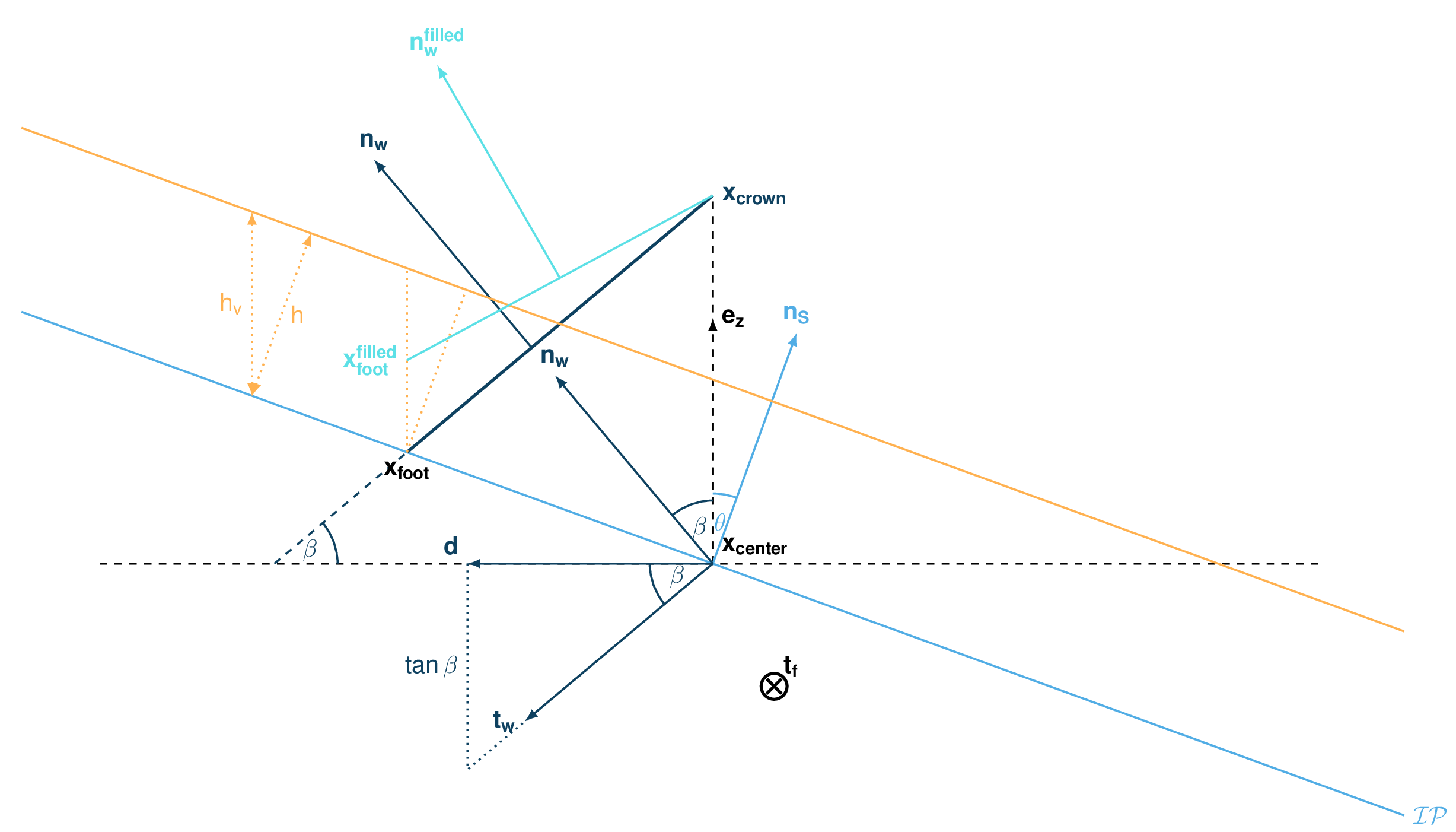
Fig. 46 Side view of the dam (cut view). \(\mathbf{x_\text{crown}}\) describes the crown of the dam, \(\mathbf{x_\text{center}}\) is the vertical projection of the crown on the topography (here the light blue line represents the topography). The tangent vector to the center line (\(\mathbf{t_f}\)) is computed from the center line points. The tangent vector to the center line with the dam slope angle enable to compute the tangent (\(\mathbf{t_w}\)) and normal (\(\mathbf{n_w}\)) vector to the dam wall. Finally, this normal vector is adjusted depending on the snow thickness at the dam location (filling of the dam , \(\mathbf{n_w^\text{filled}}\))

In the initialization of the simulation, the dam tangent vector to the center line (\(\mathbf{t_f}\)), foot line (\(\mathbf{x_\text{foot}}\)) and normal vector to the wall (\(\mathbf{n_w}\)) are computed. The grid cells crossed by the dam as well as their neighbor cells are memorized (tagged as dam cells).