com1DFA DFA-Kernel numerics
The numerical method used in com1DFA mixes particle methods and mesh methods. Mass and momentum are tracked using particles but flow thickness is tracked using the mesh. The mesh is also used to access topographic information (surface elevation, normal vector) as well as for displaying results.
Mass Eq.19 and momentum Eq.18 balance equations as well as basal normal stress Eq.17 are computed numerically using a SPH method (Smoothed Particle Hydrodynamics) ([Mon92]) for the variables \(\overline{\mathbf{u}}=(\overline{u}_1, \overline{u}_2)\) and \(\overline{h}\) by discretization of the released avalanche volume in a large number of mass elements. SPH in general, is a mesh-less numerical method for solving partial differential equations. The SPH algorithm discretizes the numerical problem within a domain using particles ([Sam07, SG09]), which interact with each-other in a defined zone of influence. Some of the advantages of the SPH method are that free surface flows, material boundaries and moving boundary conditions are considered implicitly. In addition, large deformations can be modeled due to the fact that the method is not based on a mesh. From a numerical point of view, the SPH method itself is relatively robust.
Discretization
Space discretization
The domain is discretized in particles. The following properties are assigned to each particle \(p_k\): a mass \(m_{p_k}\), a thickness \({h}_{p_k}\), a density \(\rho_{p_k}=\rho_0\) and a velocity \(\mathbf{{u}}_{p_k}=({u}_{p_k,1}, {u}_{p_k,2})\) (those quantities are thickness averaged, note that we dropped the overline from Eq.7 for simplicity reasons). In the following paragraphs, \(i\) and \(j\) indexes refer to the different directions in the NCS, whereas \(k\) and \(l\) indexes refer to particles.
The quantities velocity, mass and flow thickness are also defined on the fixed mesh. It is possible to navigate from particle property to mesh property using the interpolation methods described in Mesh and interpolation.
Time step
A fixed time step can be used or an adaptive time step that depends on the sph kernel radius as well as the particle size.
Mesh and interpolation
Here is a description of the mesh and the interpolation method that is used to switch from particle to mesh values and the other way around.
Mesh
For practical reasons, a 2D rectilinear mesh (grid) is used. Indeed the topographic input information is read from 2D raster files (with \(N_{y}\) and \(N_{x}\) rows and columns) which correspond exactly to a 2D rectilinear mesh. Moreover, as we will see in the following sections, 2D rectilinear meshes are very convenient for interpolations as well as for particle tracking. The 2D rectilinear mesh is composed of \(N_{y}\) and \(N_{x}\) rows and columns of square cells (of side length \(csz\)) and \(N_{y}+1\) and \(N_{x}+1\) rows and columns of vertices as described in Fig. 47. Each cell has a center and four vertices. The data read from the raster file is assigned to the cell centers. Note that although this is a 2D mesh, as we use a terrain-following coordinate system to perform our computations, this 2D mesh is oriented in 3D space and hence the projected side length corresponds to \(csz\), whereas the actual side length and hence also the Cell area, depend on the local slope, expressed by the Cell normals.
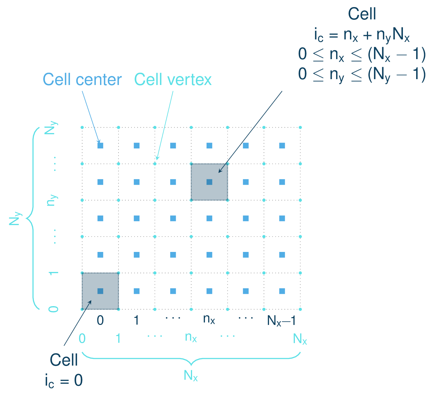
Fig. 47 Rectangular grid
Cell normals
There are many different methods available for computing normal vectors on a 2D rectilinear mesh. Several options are available in com1DFA.
The first one consists in computing the cross product of the diagonal vectors between four cell centers. This defines the normal vector at the vertices. It is then possible to interpolate the normal vector at the cell centers from the ones at the vertices.
The other methods use the plane defined by different adjacent triangles to a cell center. Each triangle has a normal and the cell center normal is the average of the triangles normal vectors.
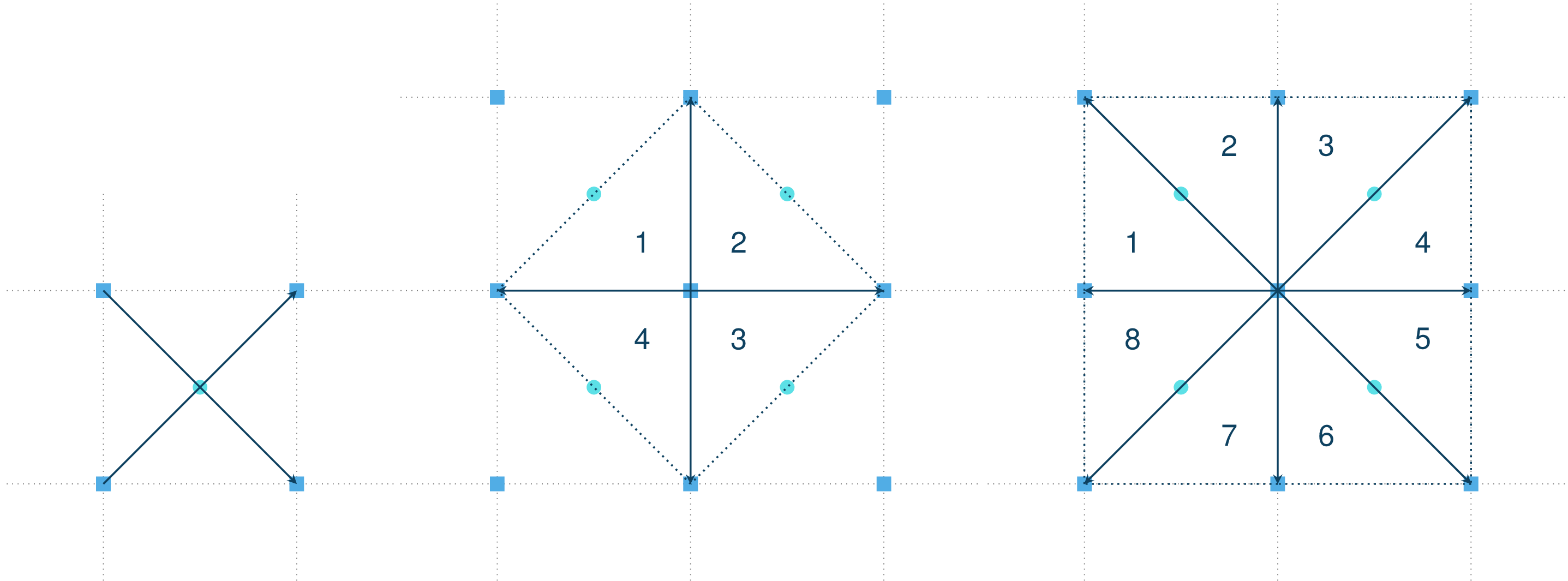
Fig. 48 Grid normal computation
Cell area
The cell area can be deduced from the grid cellsize and the cell normal. A cell is a plane (\(z = ax+by+c\)) of same normal as the cell center:
Surface integration over the cell extent leads to the area of the cell:
Interpolation
In the DFA kernel, mass, flow thickness and flow velocity can be defined at particle location or on the mesh. We need a method to be able to go from particle properties to mesh (field) values and from mesh values to particle properties.
Mesh to particle
On a 2D rectilinear mesh, scalar and vector fields defined at cell centers can be evaluated anywhere within the mesh using a bilinear interpolation between mesh cell centers. Evaluating a vector field simply consists in evaluating the three components as scalar fields.
The bilinear interpolation consists in successive linear interpolations in both \(x\) and \(y\) direction using the four nearest cell centers, two linear interpolations in the first direction (in our case in the \(y\) direction in order to evaluated \(f_{0v}\) and \(f_{1v}\)) followed by a second linear interpolation in the second direction (\(x\) in our case to finally evaluate \(f_{uv}\)) as shown on Fig. 49:
and
the \(w\) are the bilinear weights. The example given here is for a unit cell. For no unit cells, the \(u\) and \(v\) simply have to be normalized by the cell size.
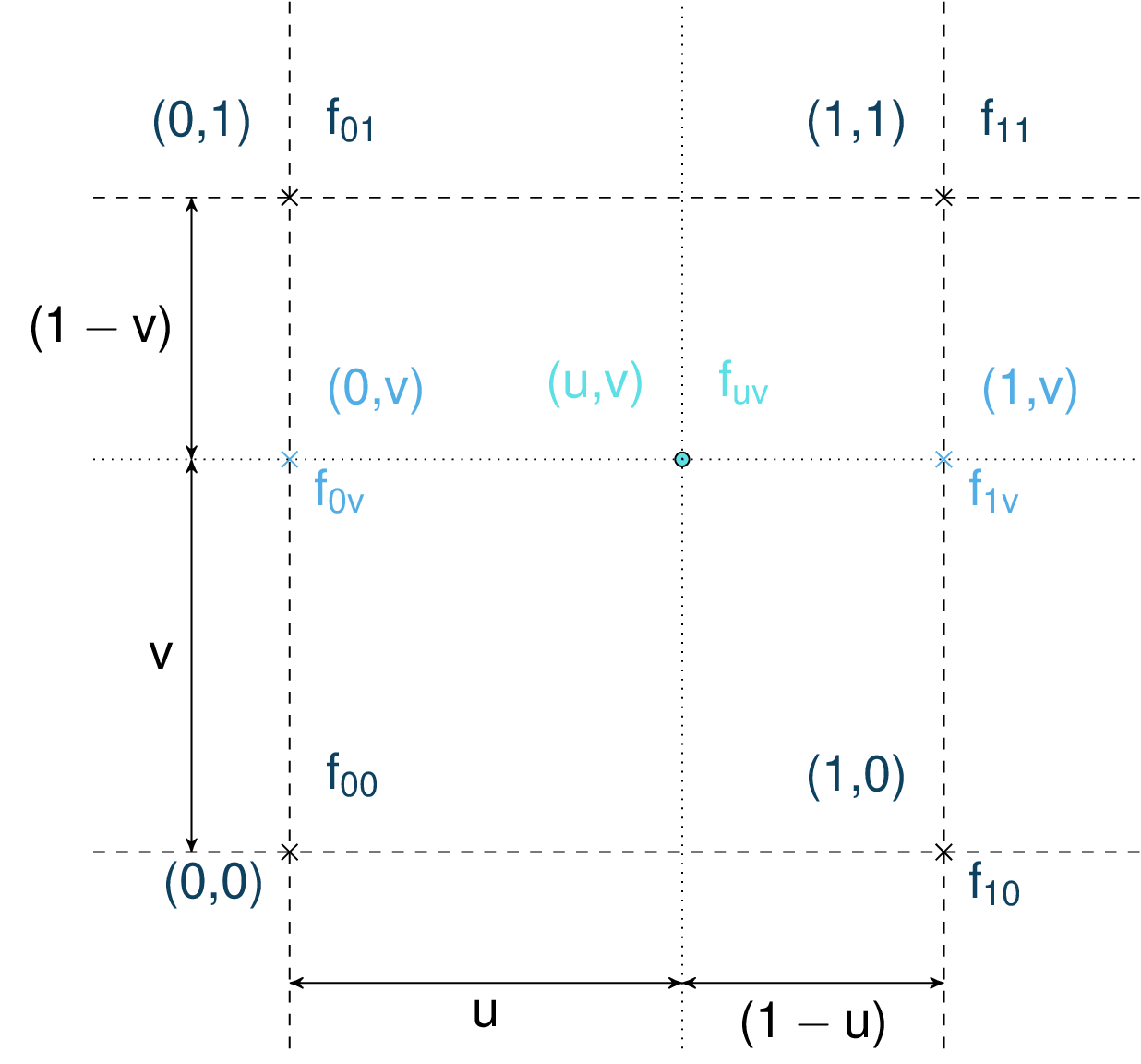
Fig. 49 Bilinear interpolation in a unit mesh (cell size is 1).
Particles to mesh
Going from particle property to mesh value is also based on bilinear interpolation and weights but requires a bit more care in order to conserve mass and momentum balance. Flow thickness and velocity fields are determined on the mesh using, as intermediate step, mass and momentum fields. First, mass and momentum mesh fields can be evaluated by summing particles mass and momentum. This can be donne using the bilinear weights \(w\) defined in the previous paragraph (here \(f\) represents the mass or momentum and \(f_{uv}\) is the particle value. \(f_{nm}\) , \({n, m} \in \{0, 1\} \times \{0, 1\}\), are the cell center values):
The contribution of each particle to the different mesh points is summed up to finally give the mesh value. This method ensures that the total mass and momentum of the particles is preserved (the mass and momentum on the mesh will sum up to the same total). Flow thickness and velocity mesh fields can then be deduced from the mass and momentum fields and the cell area (actual area of each grid cell, not the projected area).
Neighbor search
The lateral pressure forces are computed via the SPH flow thickness gradient. This method is based on particle interactions within a certain neighborhood, meaning that it is necessary to keep track of all the particles within the neighborhood of each particle. Computing the gradient of the flow thickness at a particle location, requires to find all the particles in its surrounding. Considering the number of particles and their density, computing the gradient ends up in computing a lot of interactions and represents the most computationally expensive part of the dense flow avalanche simulation. It is therefore important that the neighbor search is fast and efficient. [IOS+14] describe different rectilinear mesh neighbor search methods. In com1DFA, the simplest method is used. The idea is to locate each particle in a cell, this way, it is possible to keep track of the particles in each cell. To find the neighbors of a particle, one only needs to read the cell in which the particle is located (dark blue cell in Fig. 50) , find the direct adjacent cells in all directions (light blue cells) and simply read all particles within those cells. This is very easily achieved on rectilinear meshes because locating a particle in a cell is straightforward and finding the adjacent cells is also easily done.
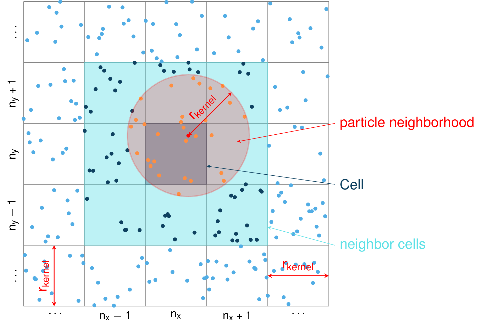
Fig. 50 Support mesh for neighbor search: if the cell side is bigger than the kernel length \(r_{kernel}\) (red circle in the picture), the neighbors for any particle in any given cell (dark blue square) can be found in the direct neighborhood of the cell itself (light blue squares)
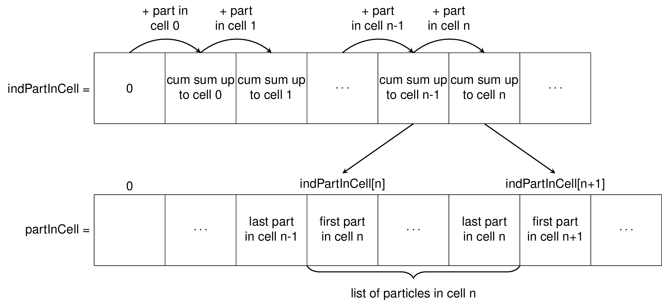
Fig. 51 The particles are located in the cells using two arrays. indPartInCell of size number of cells + 1 which keeps track of the number of particles in each cell and partInCell of size number of particles + 1 which lists the particles contained in the cells.
SPH gradient
SPH method can be used to solve thickness integrated equations where a 2D (respectively 3D) equation is reduced to a 1D (respectively 2D) one. This is used in ocean engineering to solve shallow water equations (SWE) in open or closed channels for example. In all these applications, whether it is 1D or 2D SPH, the fluid is most of the time, assumed to move on a horizontal plane (bed elevation is set to a constant). In the case of avalanche flow, the “bed” is sloped and irregular. The aim is to adapt the SPH method to apply it to thickness integrated equations on a 2D surface living in a 3D world.
Method
The SPH method is used to express a quantity (the flow thickness in our case) and its gradient at a certain particle location as a weighted sum of its neighbors properties. The principle of the method is well described in [LL10]. In the case of thickness integrated equations (for example SWE), a scalar function \(f\) and its gradient can be expressed as following:
Which gives for the flow thickness:
Where \(W\) represents the SPH-Kernel function.
The computation of its gradient depends on the coordinate system used.
Standard method
Let us start with the computation of the gradient of a scalar function \(f \colon \mathbb{R}^2 \to \mathbb{R}\) on a horizontal plane. Let \(P_k=\mathbf{x}_k=(x_{k,1},x_{k,2})\) and \(Q_l=\mathbf{x}_l=(x_{l,1},x_{l,2})\) be two points in \(\mathbb{R}^2\) defined by their coordinates in the Cartesian coordinate system \((P_k,\mathbf{e_1},\mathbf{e_2})\). \(\mathbf{r}_{kl}=\mathbf{x}_k-\mathbf{x}_l\) is the vector going from \(Q_l\) to \(P_k\) and \(r_{kl} = \left\Vert \mathbf{r}_{kl}\right\Vert\) the length of this vector. Now consider the kernel function \(W\):
In the case of the spiky kernel, \(W\) reads (2D case):
\(\left\Vert \mathbf{r_{kl}}\right\Vert= \left\Vert \mathbf{x_{k}}-\mathbf{x_{l}}\right\Vert\) represents the distance between particle \(k\) and \(l\) and \(r_0\) the smoothing length.
Using the chain rule to express the gradient of \(W\) in the Cartesian coordinate system \((x_1,x_2)\) leads to:
with,
and
which leads to the following expression for the gradient:
The gradient of \(f\) is then simply:
2.5D SPH method
We now want to express a function \(f\) and its gradient on a potentially curved surface and express this gradient in the 3 dimensional Cartesian coordinate system \((P_k,\mathbf{e_1},\mathbf{e_2},\mathbf{e_3})\).
Let us consider a smooth surface \(\mathcal{S}\) and two points \(P_k=\mathbf{x}_k=(x_{k,1},x_{k,2},x_{k,3})\) and \(Q_l=\mathbf{x}_l=(x_{l,1},x_{l,2},x_{l,3})\) on \(\mathcal{S}\). We can define \(\mathcal{TP}\) the tangent plane to \(\mathcal{S}\) in \(P_k\). If \(\mathbf{u}_k\) is the (none zero) velocity of the particle at \(P_k\), it is possible to define the local orthonormal coordinate system \((P_k,\mathbf{V_1},\mathbf{V_2},\mathbf{V_3}=\mathbf{n})\) with \(\mathbf{V_1}=\frac{\mathbf{u}_k}{\left\Vert \mathbf{u}_k\right\Vert}\) and \(\mathbf{n}\) the normal to \(\mathcal{S}\) at \(P_k\). Locally, \(\mathcal{S}\) can be assimilated to \(\mathcal{TP}\) and \(Q_l\) to its projection \(Q'_l\) on \(\mathcal{TP}\). The vector \(\mathbf{r'}_{kl}=\mathbf{x}_k-\mathbf{x'}_l\) going from \(Q'_l\) to \(P_k\) lies in \(\mathcal{TP}\) and can be express in the plane local basis:
It is important to define \(f\) properly and the gradient that will be calculated:
Indeed, since \((x_1,x_2,x_3)\) lies in \(\mathcal{TP}\), \(x_3\) is not independent of \((x_1,x_2)\):
The target is the gradient of \(\tilde{f}\) in terms of the \(\mathcal{TP}\) variables \((v_1,v_2)\). Let us call this gradient \(\mathbf{\nabla}_\mathcal{TP}\). It is then possible to apply the Standard method to compute this gradient:
Which leads to:
This gradient can now be expressed in the Cartesian coordinate system. It is clear that the change of coordinate system was not needed:
The advantage of computing the gradient in the local coordinate system is if the components (in flow direction or in cross flow direction) need to be treated differently.
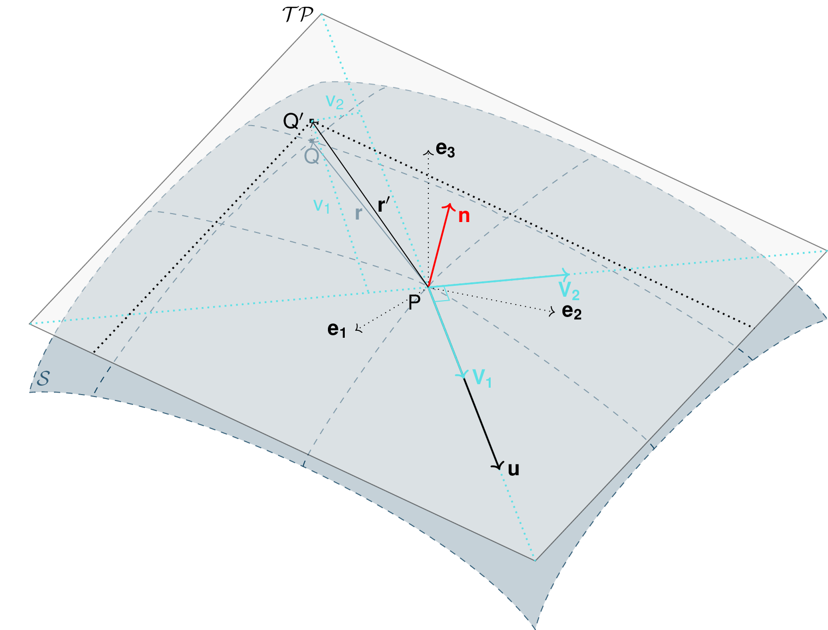
Fig. 52 Tangent plane and local coordinate system used to apply the SPH method
Particle splitting and merging
There are two different approaches treating splitting of particles in com1DFA. The first one only deals with splitting of particles with too much mass(‘split only’). The second approach, “split/merge” approach aims at keeping a stable amount of particles within a given range. This is done in order to guaranty a sufficient accuracy of the sph flow thickness gradient computation.
Split (default)
If the splitOption is set to 0, particles are split because of snow entrainment. In this case,
particles that entrain snow grow, i.e. their mass increases. At one point the mass of the particles is considered to be
too big and this particle is split in two. The splitting operation happens if the mass of the
particle exceeds a threshold value (\(mPart > massPerPart \times thresholdMassSplit\)), where thresholdMassSplit
is specified in the configuration file and massPerPart depends on the chosen massPerParticleDeterminationMethod
as defined here: Initialize particles.
When a particle is split a new child particle is created with the same properties as the parent apart from
mass and position. Both parent and child get half of the parent mass. The parent and child’s position are
adjusted: the first / second is placed forward / backward in the direction of the velocity
vector at a distance \(distSplitPart \times rPart\) of the initial parent position. Particles are considered to
have a circular basal surface \(A = \frac{m}{\rho} = \pi r^2\).
Split and merge
If the splitOption is set to 1 particles are split or merged in order to keep the particle count
as constant as possible within the kernel radius.
Assessing the number of particles within one kernel radius is done based on the particle area. Particles
are assumed to be cylindrical, i.e the base is a circle. For particle k we have \(A_k = \frac{m_k}{\rho}\). The area
of the support domain of the sph kernel function is \(\pi r_0^2\). The aim is to keep nPPK particles within
the kernel radius. The particles are split if the estimated number of particles per kernel radius \(\frac{\pi r_0^2}{A_k}\)
falls below a given value of \(n_{PPK}^{min} = C_{n_{PPK}}^{min}n_{PPK}\). Particles are split using the same
method as in Split (default). Similarly, particles are merged if the estimated
number of particles per kernel radius exceeds a given value \(n_{PPK}^{max} = C_{n_{PPK}}^{max}n_{PPK}\).
In this case particles are merged with their closest neighbor. The new position and velocity is the mass
averaged one. The new mass is the sum. Here, two coefficients \(C_{n_{PPK}}^{min}\) (cMinNPPK) and \(C_{n_{PPK}}^{max}\) (cMaxNPPK) were
introduced. A good balance needs to be found for the coefficients so that the particles are not constantly split or
merged but also not too seldom. The split and merge steps happen only once per time step and per particle.
Artificial viscosity
Two options are available to add viscosity to stabilize the numerics. The first option
consists in adding artificial viscosity (viscOption = 1). The second option attempts
to adapt the Lax-Friedrich scheme (usually applied to meshes) to the particle method
(viscOption = 2). Finally, viscOption = 0 deactivates any viscosity force.
SAMOS Artificial viscosity
In Governing Equations for the Dense Flow Avalanche, the governing equations for the DFA were derived and all first order or smaller terms where neglected. Among those terms is the lateral shear stress. This term leads toward the homogenization of the velocity field. It means that two neighbor elements of fluid should have similar velocities. The aim behind adding artificial viscosity is to take this phenomena into account. The following viscosity force is added:
Where the velocity difference reads \(\mathbf{du} = \mathbf{u} - \mathbf{\bar{u}}\) (\(\mathbf{\bar{u}}\) is the mesh velocity interpolated at the particle position). \(C_{Lat}\) is a coefficient that rules the viscous force. It would be the equivalent of \(C_{Drag}\) in the case of the drag force. The \(C_{Lat}\) is a numerical parameter that depends on the mesh size. Its value is set to 100 and should be discussed and further tested.
Adding the viscous force
The viscous force acting on particle \(k\) reads:
Updating the velocity is done in two steps. First adding the explicit term related to the mean mesh velocity and then the implicit term which leads to:
With \(C_{vis} = \frac{1}{2}\rho C_{Lat}\|\mathbf{du}_k^{old}\| A_{Lat}\frac{dt}{m}\)
Ata Artificial viscosity
An upwind method based on Lax-Friedrichs scheme
Shallow Water Equations are well known for being hyperbolic transport equations. They have the particularity of carrying discontinuities or shocks which will cause numerical instabilities.
A decentering in time allows to better capture the discontinuities. This can be done in the manner of the Lax-Friedrich scheme as described in [AS05], which is formally the same as adding a viscous force. Implementing it for the SPH method, this viscous force applied on a given particle \(k\) can be expressed as follows:
with \(\Pi_{kl} = \lambda_{kl}(\mathbf{u}_l - \mathbf{u}_k) \cdot \frac{\mathbf{r}_{kl}}{\vert\vert \mathbf{r}_{kl} \vert\vert}\), and \(\mathbf{\nabla}W_{kl}\) is the gradient of the kernel function and is described in SPH gradient.
\(\mathbf{u}_{kl} = \mathbf{u}_k - \mathbf{u}_l\) is the relative velocity between particle k and l, \(\mathbf{r}_{kl} = \mathbf{x}_k - \mathbf{x}_l\) is the vector going from particles \(l\) to particle \(k\) and \(\lambda_{kl} = \frac{c_k+c_l}{2}\) with \(c_k = \sqrt{gh_l}\) the wave speed. The \(\lambda_{kl}\) is obtained by turning expressions related to time and spatial discretization parameters into an expression on maximal speed between both particles in the Lax Friedrich scheme.
Due to the expression of the viscosity force, it makes sense to
compute it at the same place where the SPH pressure force are computed (for this reason, the
viscOption = 2 corresponding to the “Ata” viscosity option is only available
in combination with the sphOption = 2).
Forces discretization
Lateral force
The SPH method is introduced when expressing the flow thickness gradient for each particle as a weighted sum of its neighbors ([LL10, Sam07]). From now on the \(p\) for particles in \(p_k\) is dropped (same applies for \(p_l\)).
The lateral pressure forces on each particle are calculated from the compression forces on the boundary of the particle. The boundary is approximated as a square with the base side length \(\Delta s = \sqrt{A_p}\) and the respective flow height. This leads to (subscript \(|_{.,i}\) stands for the component in the \(i^{th}\) direction, \(i = {1,2}\)):
From equation Eq.18
The product of the average flow thickness \(\overline{h}\) and the basal normal pressure \(\overline{\sigma}^{(b)}_{33}\) reads (using equation Eq.17 and dropping the curvature acceleration term):
Which leads to, using the relation Eq.39:
Bottom friction force
The bottom friction forces on each particle depend on the chose friction model. Using the SamosAT friction model (using equation Eq.17 for the expression of \(\sigma^{(b)}_{k}\)) the formulation of the bottom friction forec reads:
Added resistance force
The resistance force on each particle reads:
Both the bottom friction and resistance force are friction forces. The expression above represent the maximal friction force that can be added. This maximal force is added if the particles are flowing. If not, the friction force equals the driving forces. See [MCVB+03] for more information.
In the default setup (ResistanceModel = default), either detrainment or the extra resistance force is applied within the resistance area, depending on the thickness and speed of the flow.
See theoryCom1DFA:Resistance: for more details.
Entrainment force
The term \(- \overline{u_i}\,\rho_0\,\frac{\mathrm{d}(A\,\overline{h})}{\mathrm{d}t}\) related to the entrained mass in Eq.5 now reads:
The mass of entrained snow for each particle depends on the type of entrainment involved (plowing or erosion) and reads:
with
Finaly, the entrainment force reads:
Adding forces
The different components are added following an operator splitting method. This means particle velocities are updated successively with the different forces.
Adding artificial viscosity
If the viscosity option (viscOption) is set to 1, artificial viscosity is added first, as described
in Artificial viscosity (this is the default option). With viscOption set to 0, no viscosity is added. Finally, if
viscOption is set to 2, artificial viscosity is added during SPH force computation. (TODO add link to description)
Adding entrainment
Entrainment is taken into account by first adding the component representing the loss of momentum due to acceleration of the entrained mass \(- \overline{u}_{k,i}\,A^{\text{ent}}_{k}\,q^{\text{ent}}_{k}\). Second by adding the force due to the need to break and compact the entrained mass (\(F_{k,i}^{\text{ent}}\)) as described in Entrainment force.
Adding driving forces
The driving forces -gravity force and lateral forces- are taken into account next. The velocity is updated explicitly.
Adding friction forces
Both the bottom friction and resistance forces act against the flow. Two methods are available to add these forces in com1DFA.
An implicit method:
where \(F_{k,i}^{\text{fric}} = C_{k}^{\text{fric}} u_{k,i}^{new} = F_{k,i}^{\text{res}} + F_{k,i}^{\text{bot}}\) (the two forces are described in Bottom friction force and Added resistance force).
This implicit method has a few draw-backs. First the flow does not start properly if the friction angle \(\delta\) is too close to the slope angle. Second, the flow never properly stops, even if the particles physically should, i.e. particles keep oscillating back and force around their end position.
An explicit method:
The method based on [MCVB+03] addresses these two issues. The idea is that the friction forces only modify the magnitude of velocity and not the direction. This means dissipation, so the friction force can not become a driving force. Moreover, the friction force magnitude depends on the particle state, i.e. if it is flowing or at rest. The friction force is expressed:
with:
If the velocity of the particle k reads \(\mathbf{u}_k^{old}\) after adding the driving forces, adding the
fiction force leads to :
at the condition that \(1 \geq \frac{\Delta t}{m} \frac{\|\mathbf{F}_{k}^{\text{fric}}\|_{max}}{\|\mathbf{u}^{old}_k\|}\). If on the contrary \(1 \leq \frac{\Delta t}{m} \frac{\|\mathbf{F}_{k}^{\text{fric}}\|_{max}}{\|\mathbf{u}^{old}_k\|}\), the friction would change the velocity direction which is nonphysical. In this case, the particle will stop before the end of the time step. This allows the particles to start and stop flowing properly.