ana5Utils

Automated path generation

Computational modules such as com2AB: Alpha Beta Model, com3Hybrid: Hybrid modeling, and analysis modules like ana3AIMEC: Aimec or the Distance-Time Analysis (ana5Utils) require a two-dimensional avalanche path (thalweg) and a split point as input. This thalweg and split point are usually created manually based on expert opinion. The aim of this module is to automatically generate an avalanche path from a dense flow avalanche (DFA) simulation and place a split point. The path is generated from the center of mass position of the dense material, hence referred to as the “mass- averaged path”. This mass-averaged path is then extended towards the top of the release area and at the bottom, resulting in a path that covers the entire length of the avalanche with additional buffer in the runout area. The split point is determined by fitting a parabola to the avalanche path profile.

Input

The automatic path generation requires results from dense flow simulations as input. These results can either be flow mass and thickness, or particle results from multiple simulation time steps. Com1DFA already provides these in the correct format.

We provide runAna5DFAPathGeneration, in which two main options exist:

1. Default option: Use com1DFA to generate the simulation results before generating a path. The runDFAModule flag in DFAPathGenerationCfg.ini is set to True. The default configuration for com1DFA is read, with overrides for the following settings: tSteps, resType, simTypeList, and dt.

2. DFA simulation results already exist: in this case, you may want to provide these as inputs to the path generation function. To do this, set the runDFAModule flag in DFAPathGenerationCfg.ini to False. Ensure that the avalanche directory contains Outputs/com1DFA with one or more simulation results. Additionally, the simulation DEM must be available.

Output

A mass-averaged path and corresponding split point are produced for each com1DFA simulation. These are saved as shapefiles to avalancheDir/Outputs/ana5Utils/DFAPath, in addition to a plot showing how the path was generated (see example figure below).

Fig. 33 runAna5DFAPathGeneration output plot example.

Additionally, if runDFAModule is set to True, com1DFA results with adjusted parameters are generated and saved to avalancheDir/Outputs/com1DFA.

To run

1. go to AvaFrame/avaframe

   cd avaframe
   

2. copy ana5Utils/DFAPathGenerationCfg.ini to ana5Utils/local_DFAPathGenerationCfg.ini and edit (if not, default values are used)

3. run:

   pixi run python runAna5DFAPathGeneration.py
   

Theory

Mass-averaged path

Any DFA simulation should be able to produce information about mass distribution for different time steps of the simulation (either flow thickness, mass, velocities… rasters or particles). This information is used to compute time dependent mass-averaged quantities such as position (center of mass), velocity… For a flow quantity \(\mathbf{a}(\mathbf{x}, t)\), the associated mass-averaged quantity is defined by:

\[\bar{\mathbf{a}}(t) = \frac{1}{M_V(t)} \ \int\limits_V \rho \mathbf{a}(\mathbf{x}, t)\,dV \approx \frac{\sum\limits_k m_k(t) \mathbf{a}_k(t)}{\sum\limits_k m_k(t)}\]

where \(m_k\) respectively \(\mathbf{a}_k(t)\) defines the mass respectively flow quantity of particle or raster cell \(k\). \(M_V(t)\) is the total flow mass in timestep t. Applying the mass-averaging to \((x, y, z)\) gives the mass-averaged path profile.

Note

The mass-averaged path profiles does not necessarily lie on the topography

It is also possible to compute the mass-averaged velocity squared \(\overline{\mathbf{u^2}}(t)\), kinetic energy \(\overline{\frac{1}{2}m\mathbf{u^2}}(t)\) or travel distance \(s\) (which are used in the Energy line test).

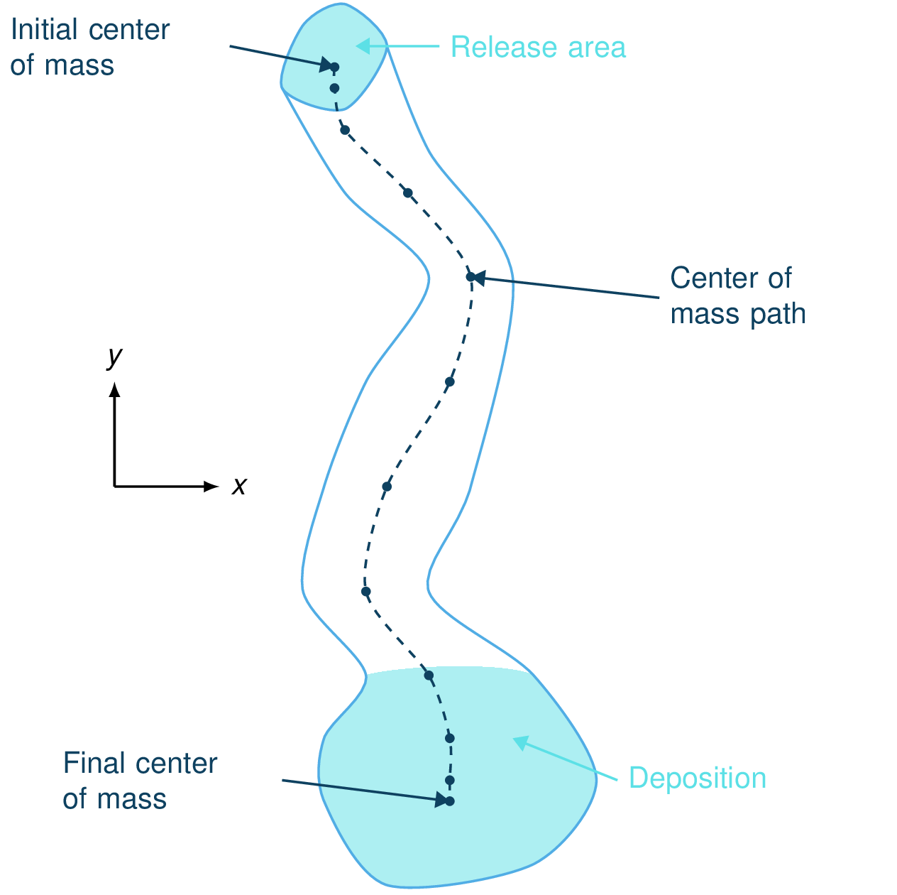
Fig. 34 Schematic showing how the mass-averaged path is generated.

Path extension

The mass-averaged path is extended towards the top of the release area to produce meaningful results when used in modules such as com2AB. Since the outcomes from the \(\alpha\beta\) analysis depend on the starting point of the path profile, adjusting the starting point will shift the \(\alpha\) angle upwards or downwards, subsequently affecting the runout value.

There are two options available to extend the mass-averaged path profile in the release area (extTopOption in the configuration file):

0. Extend the path up to the highest point in the release (highest particle or highest cell depending on which particles or rasters are available).

1. Extend the path towards the point that will lead to the longest runout. This point does not necessarily coincide with the highest point in the release area and corresponds to the point for which \((\Delta z - \Delta s \tan{\alpha})\) is maximum. \(\alpha\) corresponds to the angle of the runout line going from first to last point of the mass-averaged line. \(\Delta z\) and \(\Delta s\) represent the vertical and horizontal distance between a point in the release and the first point of the mass-averaged path profile.

We also extend the path at the bottom, to have some buffer in the runout area. This is done by finding the direction of the path given by the last few points within the path in the x,y domain (all points at a distance nCellsMinExtend * cellSize < distance < nCellsMaxExtend * cellSize)) and extending in this direction by a given factor (factBottomExt) of the total length of the path \(s\).

Resampling

If the center of mass positions are derived in an equal time interval from the simulations, derived points will not be spaced equally due to variations in flow velocity. Especially in the release and runout area, lower velocites result in a denser spacing of extracted centers of mass, which can cause a crossing of grid lines that are drawn perpendicularly to the thalweg over the width of the domain. In order to reduce these overlaps, a resampling function is used, where the thalweg is generated based on a spline of degree k (scipy splprep) and a user defined approximate distance nCellsResample between points along the spline. The path is resampled at nCellsResample * cellSize.

Split point generation

A split point is required as input for computational models such as com2AB, to define a threshold below which to look for the \(\beta\)-point. To generate this split point, a parabolic curve is fitted to the non-extended avalanche path profile extracted from the DFA simulation, ensuring that the first and last points of the parabolic profile match the avalanche path profile. To find the best fitting parabolic profile, an additional constraint is needed, where we provide two options:

1. Default Option (fitOption= 0): Minimizes the distance between the parabolic profile and the avalanche path profile.

2. Second Option (fitOption= 1): Matches the slope at the end of the parabolic curve to the avalanche path profile.

This parabolic fit determines the split point location. It is the first point for which the slope is lower than the slopeSplitPoint angle. This point is then projected on the avalanche path profile.

Distance-Time Analysis

With the functions gathered in this module, flow variables of avalanche simulation results can be visualized in a distance versus time diagram, the so called thalweg-time diagram. The tt-diagram provides a way to identify main features of the temporal evolution of flow variables along the avalanche path. This is based on the ideas presented in [FFGS13] and [RK20], where avalanche simulation results have been transformed into the radar coordinate system to facilitate direct comparison, combined with the attempt to analyze simulation results in an avalanche path dependent coordinate system ([Fis13]). In addition to the tt-diagram, ana5Utils.distanceTimeAnalysis also offers the possibility to produce simulated range-time diagrams of the flow variables with respect to a radar field of view. With this, simulation results can be directly compared to radar measurements (for example moving-target-identification (MTI) images from [KMS18]) in terms of front position and inferred approach velocity. The color-coding of the simulated range-time diagrams show the average values of the chosen flow parameter (e.g. flow thickness (FT), flow velocity (FV)) at specified range gates. This color-coding is not directly comparable to the MTI intensity given in the range-time diagram from radar measurements.

Note

The data processing for the tt-diagram and the range-time diagram can be done during run time of com1DFA, or as a postprocessing step. However, the second option requires first saving and then reading all the required time steps of the flow variable fields, which is much more computationally expensive compared to the first option.

To run

During run-time of com1DFA:

• in your local copy of com1DFA/com1DFACfg.ini in [VISUALISATION] set createRangeTimeDiagram to True and choose if you want a TTdiagram by setting this flag to True or in the case of a simulated range-time diagram to False

• in your local copy of ana5Utils/distanceTimeAnalysisCfg.ini you can adjust the default settings for the generation of the diagrams

• run runCom1DFA.py to calculate mtiInfo dictionary (saved as pickle in avalancheDir/Outputs/com1DFA/distanceTimeAnalysis/mtiInfo_simHash.p) that contains the required data for producing the tt-diagram or range-time diagram

• run runScripts.runThalwegTimeDiagram.py or runScripts.runRangeTimeDiagram.py and set the preProcessedData flag to True

As a postprocessing step:

• first you need to run com1DFA to produce fields of the desired flow variable (e.g. FT, FV) of sufficient temporal resolution (every second), for this in your local copy of com1DFACfg.ini add e.g. FT to the resType and change the tSteps to 0:1

• have a look at runScripts.runThalwegTimeDiagram.py and runScripts.runRangeTimeDiagram.py

• in your local copy of ana5Utils/distanceTimeAnalysisCfg.ini you can adjust the default settings for the generation of the diagrams

Using result fields from another module than com1DFA:

• provide name of comModule in the user input part of runScripts.runThalwegTimeDiagram.py

• save your result files for FV or FT in avalancheDirectory/Outputs/comModule/peakFiles/timesteps and the peak files for the corresponding simulation and result type to avalancheDirectory/Outputs/comModule/peakFiles.

• file names have to be of this format: A_B_C_D_E., where:

  • A - releaseAreaScenario: refers to the name of the release shape file

  • B - simulationID: needs to be unique for the respective simulation

  • C - simType: refers to null (no entrainment, no resistance), ent (with entrainment), res (with resistance), entres (with entrainment and resistance)

  • D - modelType: can be any descriptive string of the employed model (here dfa for dense flow avalanche)

  • E - result type: is pft (peak flow thickness) and pfv (peak flow velocity)

The resulting figures are saved to avalancheDirectory/Outputs/ana5Utils.

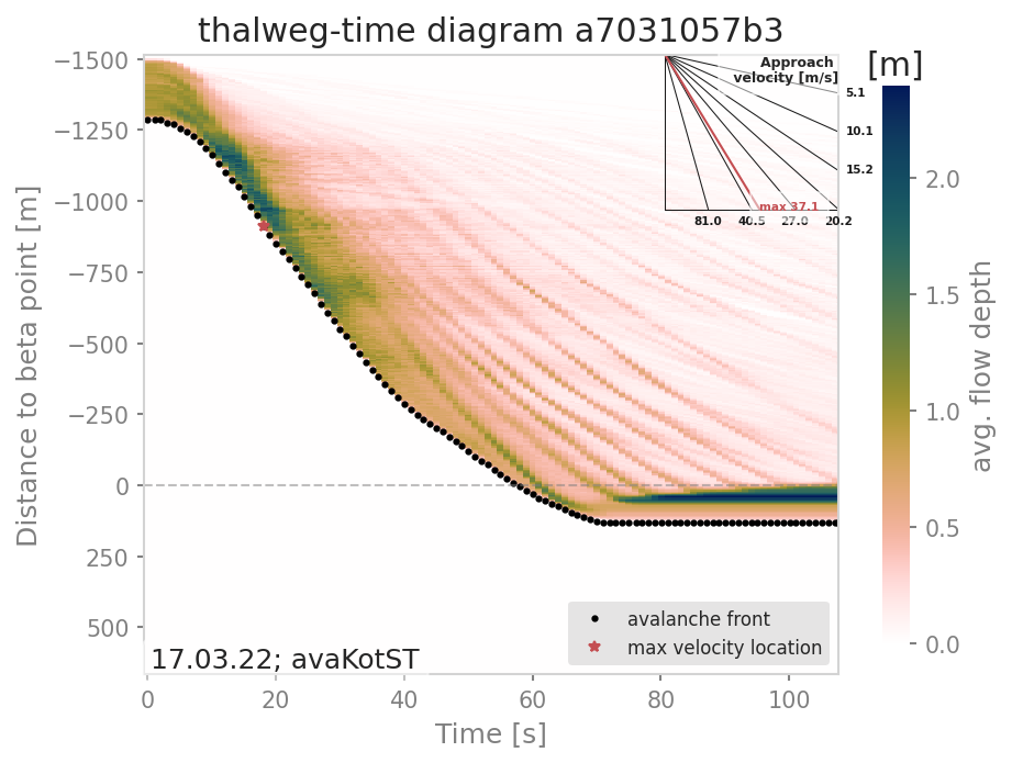
Fig. 35 Thalweg-time diagram example: The y-axis contains the distance from the beta point along the avalanche path (projected on the horizontal plane), e.g. the thalweg. Dots represent the avalanche front with the slope being the approach velocity. Red star marks the maximal approach velocity (this approach velocity is also projected on the horizontal plane).

Note

The tt-diagram requires info on an avalanche path (see ana3AIMEC: Aimec). The simulated range-time diagram requires info on the coordinates of the radar location (x0, y0), a point in the direction of the field of view (x1, y1), the aperture angle and the width of the range gates. The maximum approach velocity is indicated in the distance-time diagrams with a red star and is computed as the ratio of the distance traveled by the front and the respective time needed for a time step difference of at least minVelTimeStep which is set to 2 seconds as default. The approach velocity is a projection on the horizontal plane since the distance traveled by the front is also measured in this same plane.

Theory

Thalweg-time diagram

First, the flow variable result field is transformed into a path-following coordinate system, of which the centerline is the avalanche path. For this step, functions from ana3AIMEC are used. The distance of the avalanche front to the start of runout area point is determined using a user defined threshold of the flow variable. The front positions defined with this method for all the time steps are shown as black dots in the tt-diagram. The mean values of the flow variable are computed at cross profiles along the avalanche path for each time step and included in the tt-diagram as colored field. When computing the mean values, all the area where the flow variable is bigger than zero is taken into account. For this analysis, all available flow variables can be chosen, but the interpretation of the tt-diagram structures and the corresponding meaning of avalanche front may be different for flow thickness or flow velocity.

Simulated Range-Time diagram

The radar’s field of view is determined using its location, a point in the direction of the field of view and the horizontal (azimuth) aperture angle of the antenna. The elevation or vertical aperture angle is not yet included. The line-of-sight distance of every grid point in the simulation results to the radar location is computed. The simulation results which lie outside the radar’s field of view are masked. The distance of the avalanche front with respect to the radar location is determined for a user defined threshold in the flow variable and the average values of the result field for each range gate along the radar’s line of sight are computed. This data is plotted in a range-time diagram, where the black dots indicate the avalanche front, and the colored field indicates the mean values of the flow variable for the range gates at each time step.