com1DFA DFA-Kernel numerics

Warning

This theory has not been fully reviewed yet.

Mesh and interpolation

The numerical method used in com1DFA mixes particle methods and mesh methods. Mass and momentum are tracked using particles but flow depth is tracked using the mesh. The mesh is also to access topographic information (surface elevation, normal vector) as well as for displaying results. Here is a description of the mesh and the interpolation method used to switch from particle to mesh values and the other way around.

Mesh

For practical reasons, a 2D rectilinear mesh (grid) is used. Indeed the topographic input information is read from 2D raster files (with \(N_{y}\) and \(N_{x}\) rows and columns) which corresponds exactly to a 2D rectilinear mesh. Moreover, as we will see in the following sections, 2D rectilinear meshes are very convenient for interpolations as well as for particle tracking. The 2D rectilinear mesh is composed of \(N_{y}-1\) and \(N_{x}-1\) rows and columns of square cells (of side length \(csz\)) and \(N_{y}\) and \(N_{x}\) rows and columns of vertices as described in Fig. 8. Each cell has a center and four vertices. The data read from the raster file is affected to the vertices.

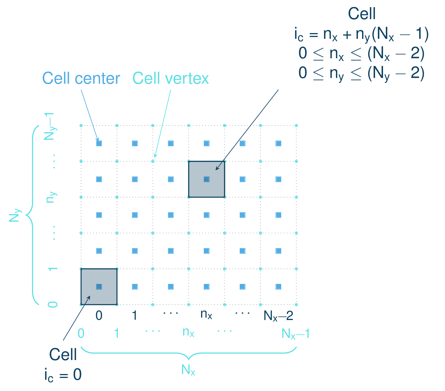
Fig. 8 Rectangular grid

Cell normals

There are many different methods available for computing normal vectors on a 2D rectilinear mesh. Several options are available in com1DFA.

The first one consists in computing the cross product of the diagonal vectors between four vertices. This defines the normal vector at the cell center. It is then possible to interpolate the normal vector at the vertices from the ones at the cell centers.

The other methods use the plane defined by the different adjacent triangles to a vertex. Each triangle has a normal and the vertices is the average of the triangles normal vectors.

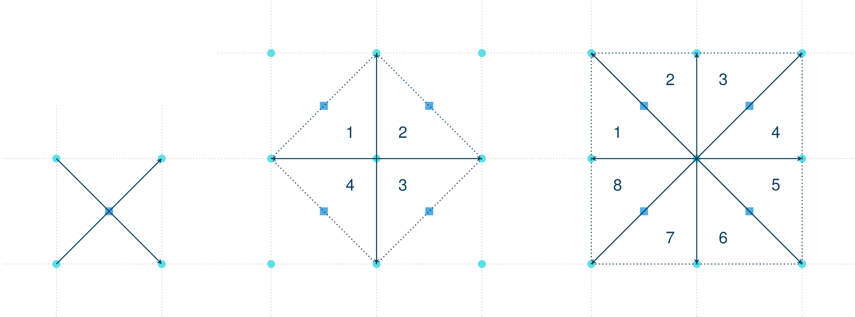
Fig. 9 Grid normal computation

Cell area

The cell area can be deduced from the grid cellsize and the cell normal. A cell is a plane (\(z = ax+by+c\)) of same normal as the cell center:

\[\begin{split}\mathbf{n} = \frac{1}{\sqrt{1+a^2+b^2}} \left|\begin{aligned} &-a\\ &-b\\ &1 \end{aligned} \right.\end{split}\]

Surface integration over the cell extend leads to the area of the cell:

\[A_{cell} = \iint_{S} \mathrm{d}{S} = \int\limits_{0}^{csz}\int\limits_{0}^{csz} \sqrt{1+\frac{\partial z}{\partial x}^2+\frac{\partial z}{\partial y}^2} \mathrm{d}{x}\,\mathrm{d}{y} = csz^2 \sqrt{1+\frac{\partial z}{\partial x}^2+\frac{\partial z}{\partial y}^2} = \frac{csz^2}{n_z}\]

The same method is used to get the area of a vertex (this does not make any sense…).

Interpolation

In the DFA kernel, mass, flow depths, velocity fields can be defined at particle location or on the mesh. We need a method to be able to go from particle property to mesh field values and from mesh values to particle property.

Mesh to particle

On a 2D rectilinear mesh, scalar and vector fields defined on mesh vertex and center can be evaluated anywhere within the mesh using a bilinear interpolation between mesh vertices. Evaluating a vector field simply consists in evaluating the three components as scalar fields.

The bilinear interpolation consists in successive linear interpolations in both \(x\) and \(y\) using the four nearest grid points, two linear interpolations in the first direction (in our case in the \(y\) direction in order to evaluated \(f_{0v}\) and \(f_{1v}\)) followed by a second linear interpolation in the second direction (\(x\) in our case to finally evaluate \(f_{uv}\)) as shown on Fig. 10:

\[\begin{split}\begin{aligned} f_{0v} = & (1-v)f_{00} + vf_{01}\\ f_{1v} = & (1-v)f_{10} + vf_{11} \end{aligned}\end{split}\]

and

\[\begin{split}\begin{aligned} f_{uv} = & (1-u)f_{0v} + uf_{1v}\\ = & (1-u)(1-v)f_{00} + (1-u)vf_{01} + u(1-v)f_{10} + uvf_{11}\\ = & w_{00}f_{00} + w_{01}f_{01} + w_{10}f_{10} + w_{11}f_{11} \end{aligned}\end{split}\]

the \(w\) are the bilinear weights. The example given here is for a unit cell. For no unit cells, the \(u\) and \(v\) simply have to be normalized by the cell size.

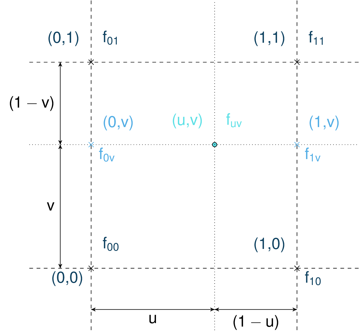
Fig. 10 Bilinear interpolation in a unit cell.

Particles to mesh

Going from particle property to mesh value is also based on bilinear interpolation and weights but requires a bit more care in order to conserve mass and momentum balance. Flow depth and velocity fields are determined on the mesh using, as intermediate step mass and momentum fields. First, mass and momentum mesh fields can be evaluated by summing particles mass and momentum. This can be donne using the bilinear weights \(w\) defined in the previous paragraph (here \(f\) represents the mass or momentum and \(f_{uv}\) is the particle value. \(f_{ij}\) are the vertex values):

\[\begin{split}\begin{aligned} f_{00} = & w_{00}f_{uv}\\ f_{01} = & w_{01}f_{uv}\\ f_{10} = & w_{10}f_{uv}\\ f_{11} = & w_{11}f_{uv} \end{aligned}\end{split}\]

The contribution of each particle to the different mesh points is summed up to finally give the mesh value. This method ensures that the total mass and momentum of the particles is preserved (the mass and momentum on the mesh will sum up to the same total). Flow depth and velocity grid fields can then be deduced from the mass and momentum fields and the cell area (real area of each grid cell).

Neighbor search

The SPH flow depth gradient computation is based on particle interactions. It requires, in order to compute the gradient of the flow depth at a particle location, to find all the particles in its surrounding. Considering the number of particles and their density, computing the gradient ends up in computing a lot of interactions and represents the most computationally expensive part of the dense flow avalanche simulation. It is therefore important that the neighbor search is fast and efficient. [IOS+14] describe different rectilinear mesh neighbor search methods. In com1DFA, the simplest method is used. The idea is to locate each particle in a cell, this way, it is possible to keep track of the particles in each cell. To find the neighbors of a particle, one only needs to read the cell in which the particle is located (dark blue cell in Fig. 11) , find the direct adjacent cells in all directions (light blue cells) and simply read all particles within those cells. This is very easily achieved on rectilinear meshes because locating a particle in a cell is straightforward and finding the adjacent cells is also immediate.

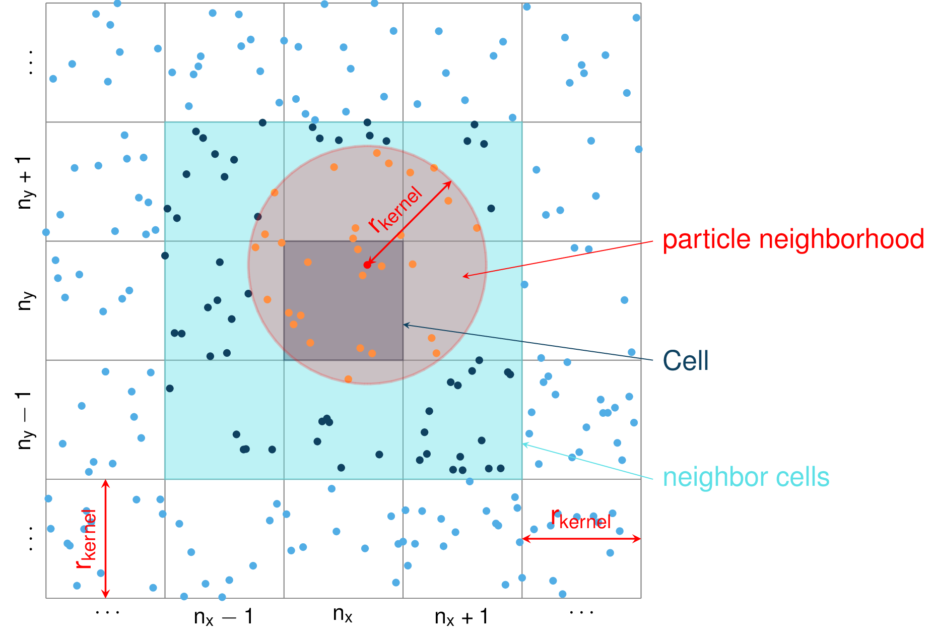
Fig. 11 Support mesh for neighbor search: if the cell side is bigger than the kernel length \(r_{kernel}\) (red circle in the picture), the neighbors for any particle in any given cell (dark blue square) can be found in the direct neighborhood of the cell itself (light blue squares)

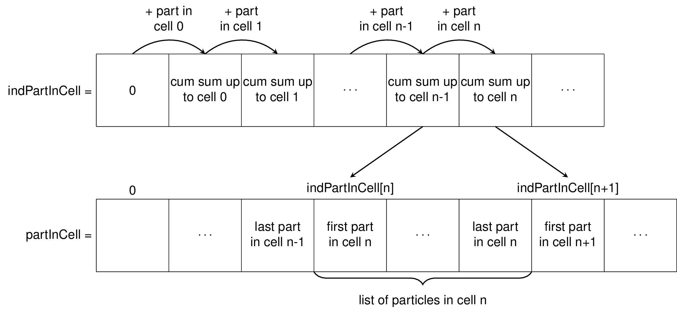
Fig. 12 The particles are located in the cells using tow arrays. indPartInCell of size number of cells + 1 which keeps track of the number of particles in each cell and partInCell of size number of particles + 1 which lists the particles contained in the cells.

SPH gradient

SPH method can be used to solve depth integrated equations where a 2D (respectively 3D) equation is reduced to a 1D (respectively 2D) one. This is used in ocean engineering to solve shallow water equations (SWE) in open or closed channels for example. In all these applications, whether it is 1D or 2D SPH, the fluid is most of the time, assumed to move on a horizontal plane (bed elevation is set to a constant). In the case of avalanche flow, the “bed” is sloped and irregular. The aim is to adapt the SPH method to apply it to depth integrated equations on a 2D surface living in a 3D world.

Method

The SPH method is used to express a quantity (the flow depth in our case) and its gradient at a certain particle location as a weighted sum of its neighbors properties. The principle of the method is well described in [LL10]. In the case a depth integrated equations (for example SWE), a scalar function \(f\) and its gradient can be expressed as following:

(23)\[\begin{split}f_{i} &= \sum\limits_{j}f_{j}A_{j}\,W_{ij}\\ \mathbf{\nabla}f_{i} &= -\sum\limits_{j}f_{j}A_{j}\,\mathbf{\nabla}W_{ij}\end{split}\]

Which gives for the flow depth:

(24)\[\begin{split}\overline{h}_{i} &= \frac{1}{\rho_0}\,\sum\limits_{j}{m_{j}}\,W_{ij}\\ \mathbf{\nabla}\overline{h}_{i} &= -\frac{1}{\rho_0}\,\sum\limits_{j}{m_{j}}\,\mathbf{\nabla}W_{ij}\end{split}\]

Where \(W\) represents the SPH-Kernel function.

The computation of its gradient depends on the coordinate system used.

Standard method

Let us start with the computation of the gradient of a scalar function \(f \colon \mathbb{R}^2 \to \mathbb{R}\) on a horizontal plane. Let \(P_i=\mathbf{x}_i=(x_{i,1},x_{i,2})\) and \(Q_j=\mathbf{x}_j=(x_{j,1},x_{j,2})\) be two points in \(\mathbb{R}^2\) defined by their coordinates in the Cartesian coordinate system \((P_i,\mathbf{e_1},\mathbf{e_2})\). \(\mathbf{r}_{ij}=\mathbf{x}_i-\mathbf{x}_j\) is the vector going from \(Q_j\) to \(P_i\) and \(r_{ij} = \left\Vert \mathbf{r}_{ij}\right\Vert\) the length of this vector. Now consider the kernel function \(W\):

\[\begin{split}\left. \begin{aligned} W \colon \mathbb{R}^2 \times \mathbb{R}^2 \times \mathbb{R} &\to \mathbb{R}\\ (P_i, Q_j, r_0) &\mapsto W(P_i, Q_j, r_0) \end{aligned} \right.\quad, r_0\in\mathbb{R} \mbox{ is the smoothing kernel length}\end{split}\]

In the case of the spiky kernel, \(W\) reads (2D case):

(25)\[\begin{split}\begin{aligned} W_{ij} = &W(\mathbf{x_i},\mathbf{x_j},r_0) = W(\mathbf{x_i}-\mathbf{x_j},r_0) = W(\mathbf{r_{ij}},r_0)\\ =&\frac{10}{\pi r_0^5}\left\{ \begin{aligned} & (r_0 - \left\Vert \mathbf{r_{ij}}\right\Vert)^3, \quad &0\leq \left\Vert \mathbf{r_{lj}}\right\Vert \leq r_0\\ & 0 , & r_0 <\left\Vert \mathbf{r_{ij}}\right\Vert \end{aligned} \right. \end{aligned}\end{split}\]

\(\left\Vert \mathbf{r_{ij}}\right\Vert= \left\Vert \mathbf{x_{i}}-\mathbf{x_{j}}\right\Vert\) represents the distance between particle \(i\) and \(j\) and \(r_0\) the smoothing length.

Using the chain rule to express the gradient of \(W\) in the Cartesian coordinate system \((x_1,x_2)\) leads to:

(26)\[\mathbf{\nabla}W_{ij} = \frac{\partial W}{\partial r}.\mathbf{\nabla}r, \quad r = \left\Vert \mathbf{r} \right\Vert = \sqrt{(x_{i,1}-x_{j,1})^2 + (x_{i,2}-x_{j,2})^2}\]

with,

\[\begin{split}\frac{\partial W}{\partial r} = -3\frac{10}{\pi r_0^5}\left\{ \begin{aligned} & (r_0 - \left\Vert \mathbf{r_{ij}}\right\Vert)^2, \quad &0\leq \left\Vert \mathbf{r_{lj}}\right\Vert \leq r_0\\ & 0 , & r_0 <\left\Vert \mathbf{r_{ij}}\right\Vert \end{aligned} \right.\end{split}\]

and

\[\frac{\partial r}{\partial w_{i,k}} = \frac{(x_{i,k}-x_{j,k})}{\sqrt{(x_{i,1}-x_{j,1})^2 + (x_{i,2}-x_{j,2})^2}}, \quad k=\{1,2\}\]

which leads to the following expression for the gradient:

(27)\[\begin{split}\mathbf{\nabla}W_{ij} = -3\frac{10}{\pi r_0^5}\left\{ \begin{aligned} & (r_0 - \left\Vert \mathbf{r_{ij}}\right\Vert)^2\frac{\mathbf{r_{ij}}}{r_{ij}}, \quad &0\leq \left\Vert \mathbf{r_{lj}}\right\Vert \leq r_0\\ & 0 , & r_0 <\left\Vert \mathbf{r_{ij}}\right\Vert \end{aligned} \right.\end{split}\]

The gradient of \(f\) is then simply:

(31)\[\mathbf{\nabla}f_{i} = -\sum\limits_{j}f_{j}A_{j}\,\mathbf{\nabla}W_{ij}\]

2.5D SPH method

We now want to express a function \(f\) and its gradient on a potentially curved surface and express this gradient in the 3 dimensional Cartesian coordinate system \((P_i,\mathbf{e_1},\mathbf{e_2},\mathbf{e_3})\).

Let us consider a smooth surface \(\mathcal{S}\) and two points \(P_i=\mathbf{x}_i=(x_{i,1},x_{i,2},x_{i,3})\) and \(Q_j=\mathbf{x}_j=(x_{j,1},x_{j,2},x_{j,3})\) on \(\mathcal{S}\). We can define \(\mathcal{TP}\) the tangent plane to \(\mathcal{S}\) in \(P_i\). If \(\mathbf{u}_i\) is the (none zero) velocity of the particle at \(P_i\), it is possible to define the local orthonormal coordinate system \((P_i,\mathbf{V_1},\mathbf{V_2},\mathbf{V_3}=\mathbf{n})\) with \(\mathbf{V_1}=\frac{\mathbf{u}_j}{\left\Vert \mathbf{u}_j\right\Vert}\) and \(\mathbf{n}\) the normal to \(\mathcal{S}\) at \(P_i\). Locally, \(\mathcal{S}\) can be assimilated to \(\mathcal{TP}\) and \(Q_j\) to its projection \(Q'_j\) on \(\mathcal{TP}\). The vector \(\mathbf{r'}_{ij}=\mathbf{x}_i-\mathbf{x'}_j\) going from \(Q'_j\) to \(P_i\) lies in \(\mathcal{TP}\) and can be express in the plane local basis:

\[\mathbf{r'}_{ij}=\mathbf{x}_i-\mathbf{x'}_j = v_{ij,1}\mathbf{V_1} + v_{ij,2}\mathbf{V_2}\]

It is important to define \(f\) properly and the gradient that will be calculated:

\[\begin{split}\left. \begin{aligned} f \colon \mathcal{TP}\subset\mathbb{R}^3 &\to \mathbb{R}\\ (x_1,x_2,x_3) &\mapsto f(x_1,x_2,x_3) = f(x_1(v_1,v_2),x_2(v_1,v_2)) = \tilde{f}(v_1,v_2) \end{aligned} \right.\end{split}\]

Indeed, since \((x_1,x_2,x_3)\) lies in \(\mathcal{TP}\), \(x_3\) is not independent of \((x_1,x_2)\):

\[\begin{split}\left. \begin{aligned} \tilde{f} \colon \mathcal{TP}\subset\mathbb{R}^2 &\to \mathbb{R}\\ (v_1,v_2) &\mapsto \tilde{f}(v_1,v_2) = \tilde{f}(v_1(x_1,x_2),v_2(x_1,x_2)) = f(x_1,x_2,x_3) \end{aligned} \right.\end{split}\]

The target is the gradient of \(\tilde{f}\) in terms of the \(\mathcal{TP}\) variables \((v_1,v_2)\). Let us call this gradient \(\mathbf{\nabla}_\mathcal{TP}\). It is then possible to apply the Standard method to compute this gradient:

(29)\[\mathbf{\nabla}_\mathcal{TP}W_{ij} = \frac{\partial W}{\partial r}.\mathbf{\nabla}_\mathcal{TP}r, \quad r = \left\Vert \mathbf{r} \right\Vert = \sqrt{v_{ij,1}^2 + v_{ij,2}^2}\]

Which leads to:

(30)\[\begin{split}\mathbf{\nabla}_\mathcal{TP}W_{ij} = -3\frac{10}{\pi r_0^5}\frac{(r_0 - \left\Vert \mathbf{r_{ij}'}\right\Vert)^2}{r_{ij}'}\left\{ \begin{aligned} & v_{ij,1}\mathbf{V_1} + v_{ij,2}\mathbf{V_2}, \quad &0\leq \left\Vert \mathbf{r_{ij}'}\right\Vert \leq r_0\\ & 0 , & r_0 <\left\Vert \mathbf{r_{ij}'}\right\Vert \end{aligned} \right.\end{split}\]

(31)\[\mathbf{\nabla}_\mathcal{TP}\tilde{f_{i}} = -\sum\limits_{j}\tilde{f_{j}}A_{j}\,\mathbf{\nabla}W_{ij}\]

This gradient can now be expressed in the Cartesian coordinate system. It is clear that the change of coordinate system was not needed:

\[\begin{split}\mathbf{\nabla}_\mathcal{TP}W_{ij} = -3\frac{10}{\pi r_0^5}\frac{(r_0 - \left\Vert \mathbf{r_{ij}'}\right\Vert)^2}{r_{ij}'}\left\{ \begin{aligned} & r_{ij,1}\mathbf{e_1} + r_{ij,2}\mathbf{e_2} + r_{ij,3}\mathbf{e_3}, \quad &0\leq \left\Vert \mathbf{r_{ij}'}\right\Vert \leq r_0\\ & 0 , & r_0 <\left\Vert \mathbf{r_{ij}'}\right\Vert \end{aligned} \right.\end{split}\]

The advantage of computing the gradient in the local coordinate system is if the components (in flow direction or in cross flow direction) need to be treated differently.

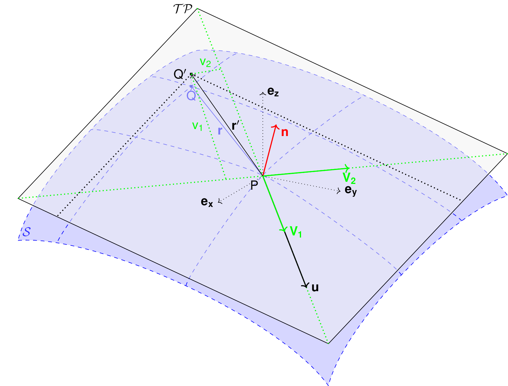
Fig. 13 Tangent plane and local coordinate system used to apply the SPH method

Artificial viscosity

Question: Why add the artificial viscosity at the beginning of the time step? makes no sense

In Governing Equations for the Dense Flow Avalanche, the governing equations for the DFA were derived and all first order or smaller terms where neglected. Among those terms is the lateral shear stress. This term leads toward the homogenization of the velocity field. It means that two neighbor elements of fluid should have similar velocities. The aim behind adding artificial viscosity is to

\[\begin{split}\begin{aligned} \mathbf{F_{viscosity}} = &- \frac{1}{2}\rho C_{Lat}\|\mathbf{du}\|^2 A_{Lat} \frac{\mathbf{du}}{\|\mathbf{du}\|}\\ = & - \frac{1}{2}\rho C_{Lat}\|\mathbf{du}\| A_{Lat} \mathbf{du} \end{aligned}\end{split}\]

Where the velocity difference reads \(\mathbf{du} = \mathbf{u} - \mathbf{\bar{u}}\) (\(\mathbf{\bar{u}}\) is the mesh velocity interpolated at the particle position). \(C_{Lat}\) is a coefficient that rules the viscous force. It would be the equivalent of \(C_{Drag}\) in the case of the drag force. The \(C_{Lat}\) is a numerical parameter that depends on the mesh size. Its value is set to 100 and should be discussed and further tested.

Adding the viscous force

The viscous force is added implicitly:

\[\begin{split}\begin{aligned} \mathbf{F_{viscosity}} = &-\frac{1}{2}\rho C_{Lat}\|\mathbf{du}^{old}\| A_{Lat} \mathbf{du}^{new}\\ = & -\frac{1}{2}\rho C_{Lat}\|\mathbf{u}^{old} - \mathbf{\bar{u}}^{old}\| A_{Lat} (\mathbf{u}^{new} - \mathbf{\bar{u}}^{old}) \end{aligned}\end{split}\]

Updating the velocity is done in two steps. First adding the explcit term related to the mean mesh velocity and then the implicit term which leads to:

\[\mathbf{u}^{new} = \frac{\mathbf{u}^{old} - C_{vis}\mathbf{\bar{u}}^{old}}{1 + C_{vis}}\]

With \(C_{vis} = \frac{1}{2}\rho C_{Lat}\|\mathbf{du}^{old}\| A_{Lat}\frac{dt}{m}\)