ana5Utils
distanceTimeAnalysis: Visualizing the temporal evolution of flow variables
With the functions gathered in this module, flow variables of avalanche simulation results can be
visualized in a distance versus time diagram, the so called thalweg-time diagram.
The tt-diagram provides a way to identify main features of the temporal evolution of
flow variables along the avalanche path.
This is based on the ideas presented in [FFGS13] and [RKohler20], where
avalanche simulation results have been transformed into the radar coordinate system to facilitate
direct comparison, combined with the attempt to analyze simulation results in an avalanche path
dependent coordinate system ([Fis13]).
In addition to the tt-diagram, ana5Utils.distanceTimeAnalysis also offers the possibility to
produce simulated range-time diagrams of the flow variables with respect to a radar field
of view. With this, simulation results can be directly compared to radar measurements (for
example moving-target-identification (MTI) images from [KohlerMS18]) in terms
of front position and inferred approach velocity. The colorcoding of the simulated
range-time diagrams show the average values of the chosen flow parameter
(e.g. flow depth (FD), flow velocity (FV)) at specified range gates. This colorcoding is not directly
comparable to the MTI intensity given in the range-time diagram from radar measurements.
Note
The data processing for the tt-diagram and the range-time diagram can be done
during run time of com1DFA, or as a postprocessing step. However, the second option
requires first saving and then reading all the required time steps of the flow variable fields,
which is much more computationally expensive compared to the first option.
To run
During run-time of com1DFA:
in your local copy of
com1DFA/com1DFACfg.iniin [VISUALISATION] set createRangeTimeDiagram to True and choose if you want a TTdiagram by setting this flag to True or in the case of a simulated range-time diagram to Falsein your local copy of
ana5Utils/distanceTimeAnalysisCfg.iniyou can adjust the default settings for the generation of the diagramsrun
runCom1DFA.pyto calculate mtiInfo dictionary (saved as pickle inavalancheDir/Outputs/com1DFA/distanceTimeAnalysis/mtiInfo_simHash.p) that contains the required data for producing the tt-diagram or range-time diagramrun
runScripts.runThalwegTimeDiagram.pyorrunScripts.runRangeTimeDiagram.pyand set the preProcessedData flag to True
As a postprocessing step:
first you need to run
com1DFAto produce fields of the desired flow variable (e.g. FD, FV) of sufficient temporal resolution (every second), for this in your local copy of com1DFACfg.ini add e.g. FD to the resType and change the tSteps to 0:1have a look at
runScripts.runThalwegTimeDiagram.pyandrunScripts.runRangeTimeDiagram.pyin your local copy of
ana5Utils/distanceTimeAnalysisCfg.iniyou can adjust the default settings for the generation of the diagrams
The resulting figures are saved to avalancheDirectory/Outputs/ana5Utils.
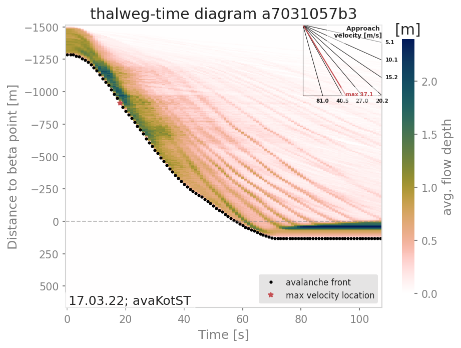
Fig. 25 Thalweg-time diagram example: The y-axis contains the distance from the beta point along the avalanche path (projected on the horizontal plane), e.g. the thalweg. Dots represent the avalanche front with the slope being the approach velocity. Red star marks the maximal approach velocity (this approach velocity is also projected on the horizontal plane).
Note
The tt-diagram requires info on an avalanche path (see ana3AIMEC: Aimec). The simulated range-time diagram requires info on the coordinates of the radar location (x0, y0), a point in the direction of the field of view (x1, y1), the aperture angle and the width of the range gates. The maximum approach velocity is indicated in the distance-time diagrams with a red star and is computed as the ratio of the distance traveled by the front and the respective time needed for a time step difference of at least minVelTimeStep which is set to 2 seconds as default. The approach velocity is a projection on the horizontal plane since the distance traveled by the front is also measured in this same plane.
Theory
Thalweg-time diagram
First, the flow variable result field is transformed into a path-following coordinate system, of
which the centerline is the avalanche path.
For this step, functions from ana3AIMEC are used.
The distance of the avalanche front to the start of runout area point is determined using a user
defined threshold of the flow variable. The front positions defined with this
method for all the time steps are shown as black dots in the tt-diagram.
The mean values of the flow variable are computed at cross profiles along the avalanche path for
each time step and included in the tt-diagram as colored field. When computing the mean values,
all the area where the flow variable is bigger than zero is taken into account.
For this analysis, all available flow variables can be chosen, but the interpretation of the
tt-diagram structures and the corresponding meaning of avalanche front may be different for
flow thickness or flow velocity.
Simulated Range-Time diagram
The radar’s field of view is determined using its location, a point in the direction of the field of view and the horizontal (azimuth) aperture angle of the antenna. The elevation or vertical aperture angle is not yet included. The line-of-sight distance of every grid point in the simulation results to the radar location is computed. The simulation results which lie outside the radar’s field of view are masked. The distance of the avalanche front with respect to the radar location is determined for a user defined threshold in the flow variable and the average values of the result field for each range gate along the radar’s line of sight are computed. This data is plotted in a range-time diagram, where the black dots indicate the avalanche front, and the colored field indicates the mean values of the flow variable for the range gates at each time step.