ana3AIMEC: Aimec

Aimec is a post-processing module to analyze and compare results from avalanche simulations. It enables the comparison of different simulations (with different input parameter sets for example, or from different models) of the same avalanche (meaning using the same DEM and going down the same avalanche path) in a standardized way.

In AvaFrame/avaframe/runScripts, three different run scripts are provided that show examples on how the postprocessing module aimec can be used. These examples include:

• full aimec analysis for simulation results of one computational module (from 1 simulation to x simulations). runScripts.runAna3AIMEC.runAna3AIMEC()

• using aimec to compare the results of two different computational modules (for one simulation at a time hence only one simulation result per computational module is passed at a time). runScripts.runAna3AIMECCompMods.runAna3AIMECCompMods()

• using aimec to compare one result parameter (ppr, pfd, pfv) for different simulations in a given inputDir (from 1 simulation to x simulations). runScripts.runAna3AIMECIndi

Here is an example workflow for the full Aimec analysis, as provided in runScripts/runAna3AIMEC.py:

Inputs

• raster of the DEM (.asc file)

• avalanche path in LINES (as a shapefile named path_aimec.shp)

• a splitPoint in POINTS (as a shapefile named splitPoint.shp)

• Results from avalanche simulation (when using results from com1DFA, the helper function ana3AIMEC.dfa2Aimec.mainDfa2Aimec() in ana3AIMEC.dfa2Aimec fetches and prepares the input for Aimec)

Note

The spatial resolution of the DEM and its extend can differ from the result raster data. However, all the result raster have to be of identical spatial resolution and extent. This might be of interest if the result rasters have been derived by remeshing the DEM to different spatial resolution. The DEM data is used to compute the z coordinate of the location of the runout point as well as the fall height (deltaH).

Outputs

• output figures in NameOfAvalanche/Outputs/ana3AIMEC/com1DFA/pics/

• txt file with results in NameOfAvalanche/Outputs/ana3AIMEC/com1DFA/

(a detailed list of the results is described in moduleAna3AIMEC.analyze-results)

To run

• first go to AvaFrame/avaframe

• copy ana3AIMEC/ana3AIMECCfg.ini to ana3AIMEC/local_ana3AIMECCfg.ini (if not, the standard settings are used)

• enter path to the desired NameOfAvalanche/ folder in your local copy of avaframeCfg.ini

• run:

  python3 runScripts/runAna3AIMEC.py
  

Theory

AIMEC (Automated Indicator based Model Evaluation and Comparison, [Fis13]) was developed to analyze and compare avalanche simulations. The computational module presented here is inspired from the original AIMEC code. The simulations are analyzed and compared by projecting the results along a chosen poly-line (same line for all the simulations that are compared) called avalanche path. The raster data, initially located on a regular and uniform grid (with coordinates x and y) is projected on a regular non uniform grid (grid points are not uniformly spaced) that follows the avalanche path (with curvilinear coordinates (s,l)). This grid can then be “straightened” or “deskewed” in order to plot it in the (s,l) coordinates system.

The simulation results (two dimensional fields of e.g. peak velocities / pressure or flow depth) are processed in a way that it is possible to compare characteristic values that are directly linked to the flow variables such as maximum peak flow depth, maximum peak velocity or deduced quantities, for example maximum peak pressure, pressure based runout (including direct comparison to possible references, see Area indicators) for different simulations. The following figure illustrates the raster transformation process.

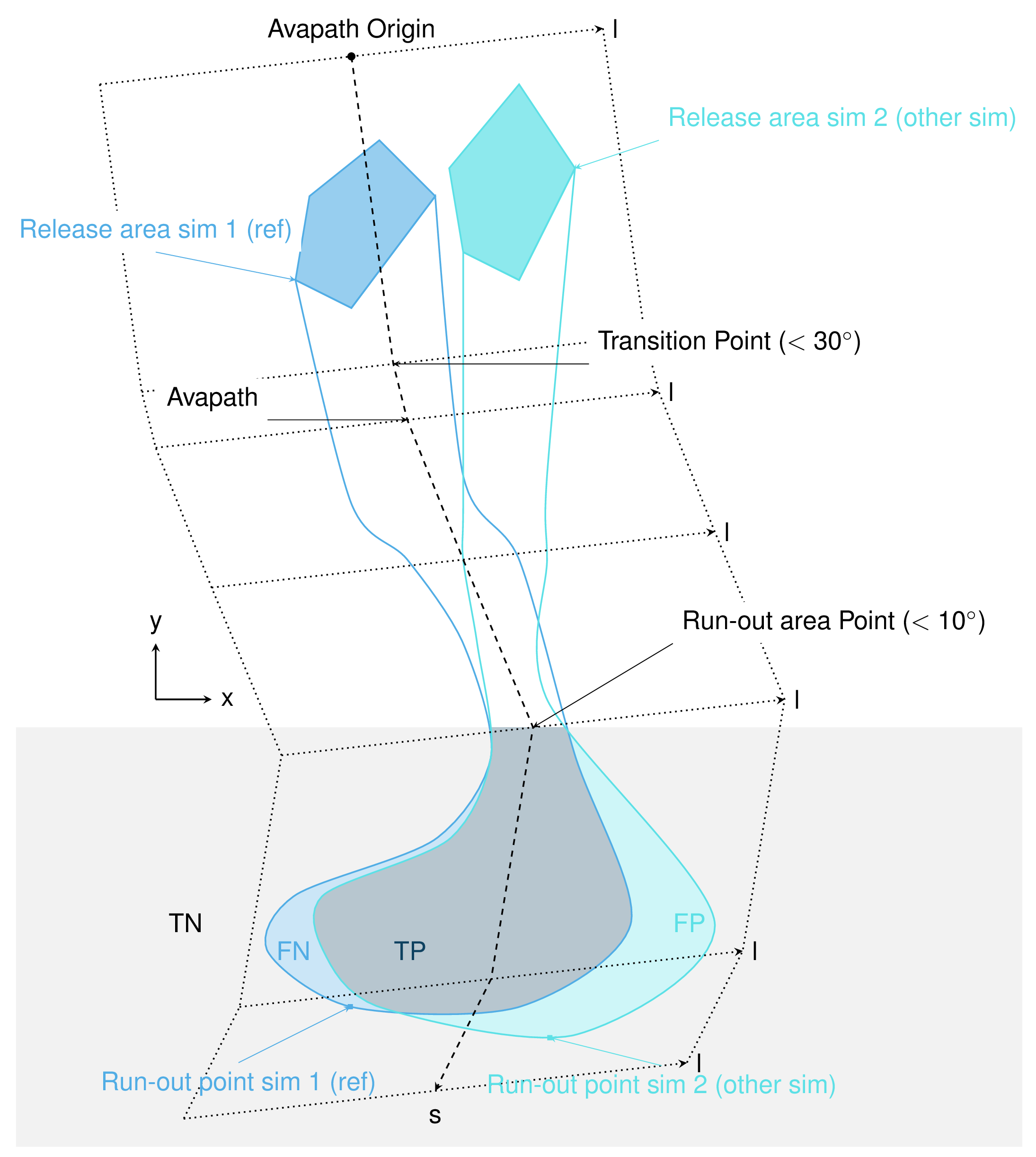
Fig. 13 In the real coordinate system (x,y)

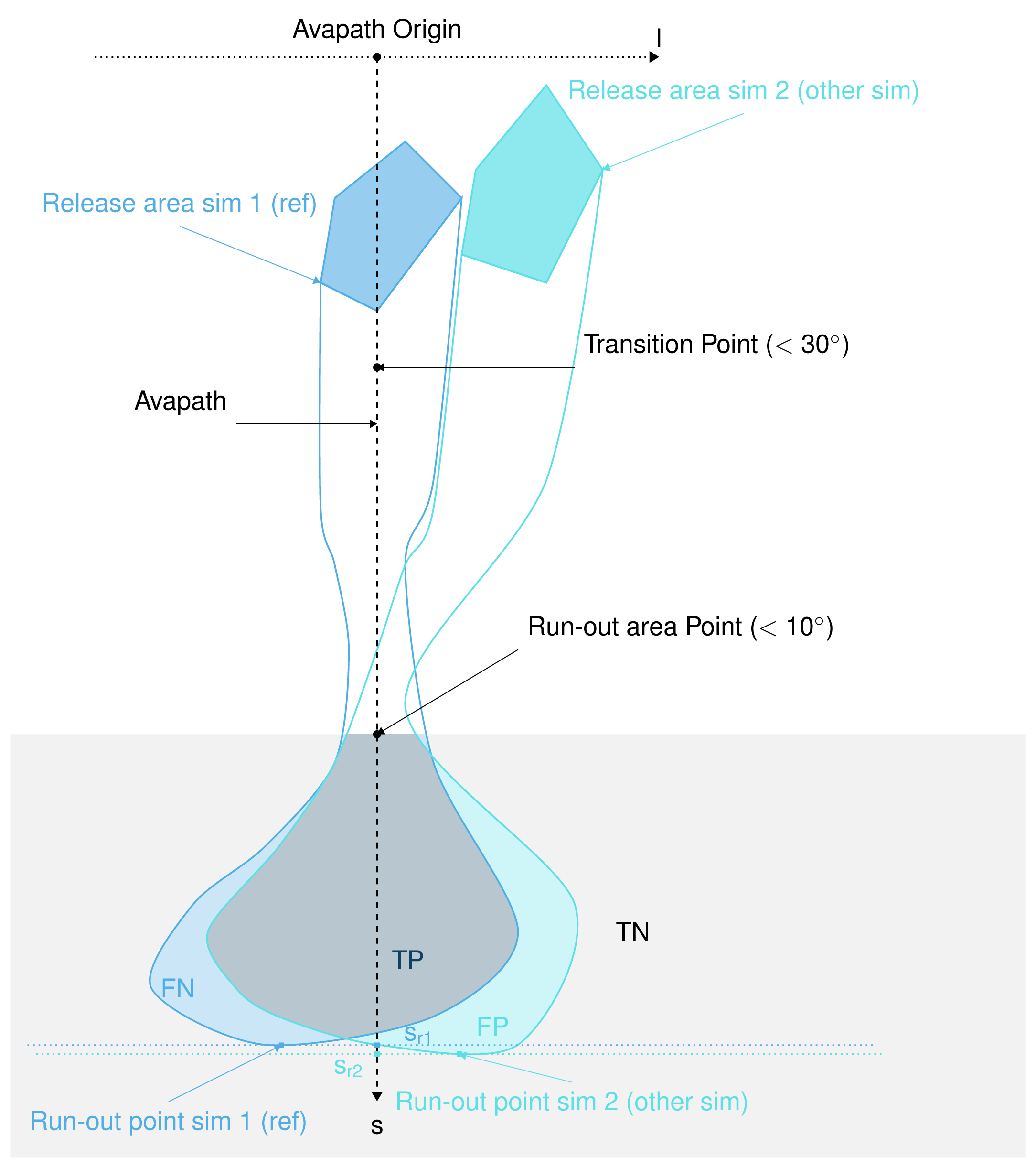
Fig. 14 In the new coordinate system (s,l)

Here is the definition of the different indicators and outputs from the AIMEC post-processing process:

Mean and max values along path

All two dimensional field results (for example peak velocities / pressure or flow depth) can be projected into the curvilinear system using the previously described method. The maximum and average values of those fields are computed in each cross-section (l direction). For example the maximum \(A_{cross}^{max}(s)\) and average \(\bar{A}_{cross}(s)\) of the two dimensional distribution \(A(s,l)\) is:

\[A_{cross}^{max}(s) = \max_{\forall l \in [-\frac{w}{2},\frac{w}{2}]} A(s,l) \quad\mbox{and}\quad \bar{A}_{cross}(s) = \frac{1}{w}\int_{-\frac{w}{2}}^{\frac{w}{2}} A(s,l)dl\]

Runout point

The runout point corresponding to a given pressure threshold \(P_{lim}>0kPa\) is the first point \(s=s_{runout}\) where the maximum peak pressure falls below the pressure limit (\(P_{cross}^{max}(s)<P_{Lim}\)). This \(s=s_{runout}\) is related to a \((x_{runout},y_{runout})\) in the original coordinate system. It is very important to note that the position of this point depends on the chosen pressure limit value. It would also be possible to use \(\bar{P}_{cross}(s)<P_{Lim}\) instead of \(P_{cross}^{max}(s)<P_{Lim}\).

Runout length

This length depends on what is considered the beginning of the avalanche \(s=s_{start}\). It can be related to the release area, to the transition point (first point where the slope angle is below \(30^{\circ}\)) or to the runout area point (first point where the slope angle is below \(10^{\circ}\)). The runout length is then defined as \(L=s_{runout}-s_{start}\).

Mean and max indicators

From the maximum values along path of the distribution \(A(s,l)\) calculated in Mean and max values along path, it is possible to calculate the global maximum (MMA) and average maximum (AMA) values of the two dimensional distribution \(A(s,l)\):

\[MMA = \max_{\forall s \in [s_{start},s_{runout}]} A_{cross}^{max}(s) \quad\mbox{and}\quad AMA = \frac{1}{s_{runout}-s_{start}}\int_{s_{start}}^{s_{runout}} A_{cross}^{max}(s)ds\]

Area indicators

When comparing the runout area (corresponding to a given pressure threshold \(P_{cross}^{max}(s)>P_{Lim}\)) of two simulations, it is possible to distinguish four different zones. For example, if the first simulation (sim1) is taken as reference and if True corresponds to the assertion that the avalanche covered this zone and False there was no avalanche in this zone, those four zones are:

• TP (true positive) zone: green zone on Fig. 14 , sim1 = True sim2 = True

• FP (false positive) zone: blue zone on Fig. 14 , sim1 = False sim2 = True

• FN (false negative) zone: red zone on Fig. 14 , sim1 = True sim2 = False

• TN (true negative) zone: gray zone on Fig. 14 , sim1 = False sim2 = False

The two simulations are identical (in the runout zone) when the area of both FP and FN is zero. In order to provide a normalized number describing the difference between two simulations, the area of the different zones is normalized by the area of the reference simulation \(A_{ref} = A_{TP} + A_{FP}\). This leads to the 4 area indicators:

• \(\alpha_{TP} = A_{TP}/A_{ref}\), which is 1 if sim2 covers at least the reference

• \(\alpha_{FP} = A_{FP}/A_{ref}\), which is a positive value if sim2 covers an area outside of the reference

• \(\alpha_{FN} = A_{FN}/A_{ref}\), which is a positive value if the reference covers an area outside of sim2

• \(\alpha_{TN} = A_{TN}/A_{ref}\)

Identical simulations (in the runout zone) lead to \(\alpha_{TP} = 1\) , \(\alpha_{FP} = 0\) and \(\alpha_{FN} = 0\)

Mass indicators

From the analysis of the release mass (\(m_r\) at the beginning, i.e \(t = t_{ini}\)), total mass (\(m_t\) at the end, i.e \(t = t_{end}\)) and entrained mass (\(m_e\) at the end, i.e \(t = t_{end}\)) it is possible to calculate the growth index \(GI\) and growth gradient \(GG\) of the avalanche:

\[GI = \frac{m_t}{m_r} = \frac{m_r + m_e}{m_r} \quad\mbox{and}\quad GG = \frac{m_r + m_e}{t_{end}-t_{ini}}\]

Time evolution of the total mass and entrained one are also analyzed.

Procedure

This section describes how the theory is implemented in the ana3AIMEC module.

Perform path-domain transformation

First, the transformation from (x,y) coordinate system (where the original rasters lie in) to (s,l) coordinate system is applied given a new domain width. This is done by ana3AIMEC.aimecTools.makeDomainTransfo(). A new grid corresponding to the new domain (following the avalanche path) is built. The transformation information are stored in a rasterTransfo dictionary (see ana3AIMEC.aimecTools.makeDomainTransfo() for more details).

Assign data

The simulation results (for example peak velocities / pressure or flow depth) are projected on the new grid using the transformation information by ana3AIMEC.aimecTools.assignData(). The projected results are stored in the newRasters dictionary.

This results in the following plot:

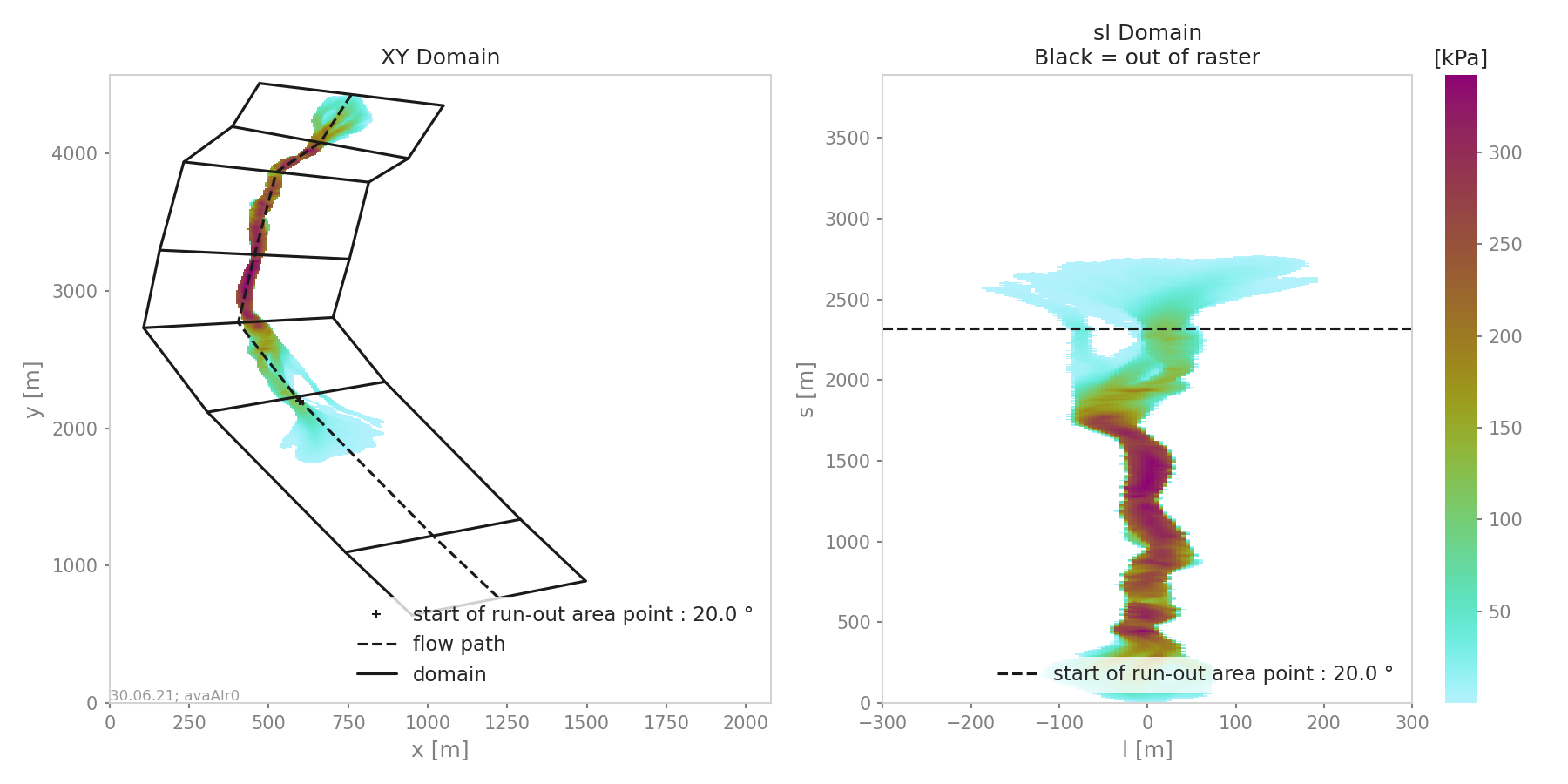
Fig. 15 Alr avalanche coordinate transformation and peak pressure field reprojetion.

Analyze results

Calculates the different indicators described in the Theory section for a given threshold. The threshold can be based on pressure, flow depth, … (this needs to be specified in the configuration file). Returns a resAnalysis dictionary with the analysis results (see ana3AIMEC.ana3AIMEC.postProcessAIMEC() for more details).

Plot and save results

Plots and saves the desired figures. Writes results in resAnalysis to a text file. By default, Aimec saves five plots plus as many plots as numerical simulations to compare to the reference. The first five ones are :

• “DomainTransformation” shows the real domain on the left and new domain on the right (Fig. 15)

• “referenceFields” shows the peak pressure, flow depth and speed in the new domain

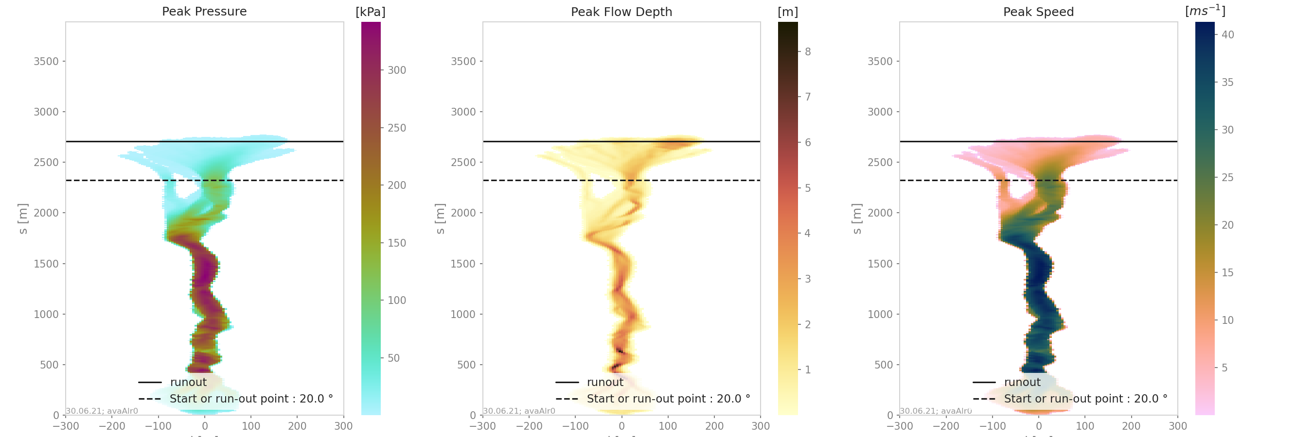
Fig. 16 Reference peak fields

• “slComparison” shows the difference between all simulations in terms of peak values along profile.

If only two simulations are provided, a 3 panel plot like the following is produced:

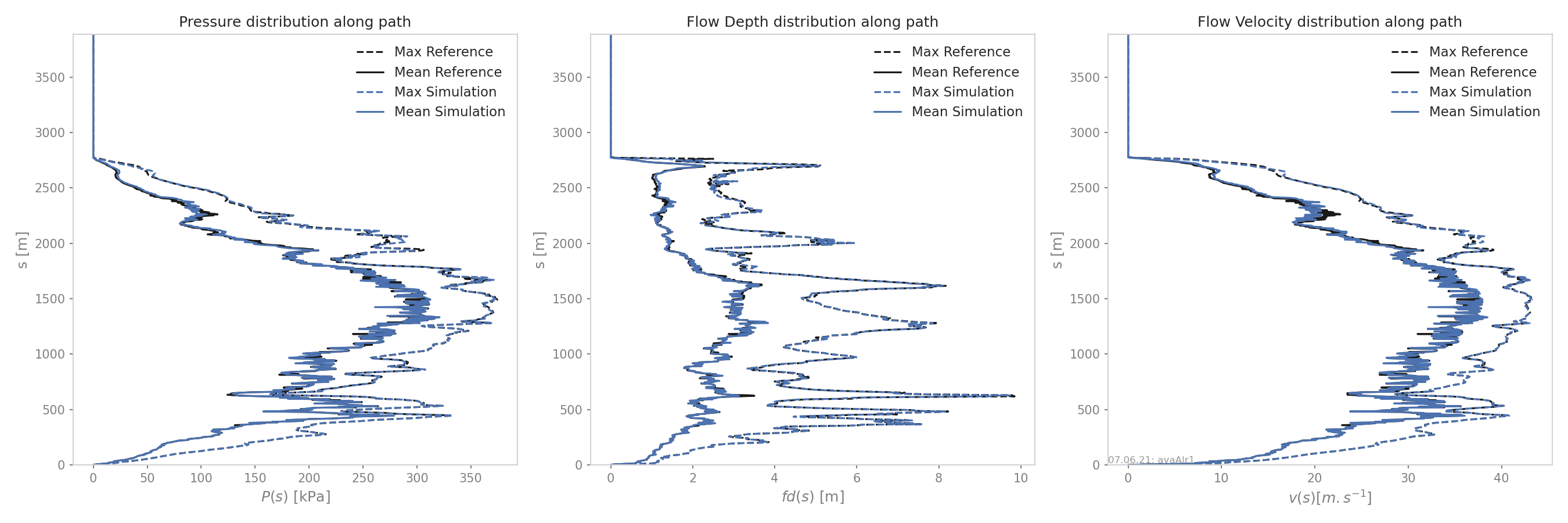
Fig. 17 Maximum peak fields comparison between two simulations

if more then two simulations are provided only the peak field specified in the configuration file is analyzed and the statistics in terms of peak value along profile are plotted (mean, max and quantiles):

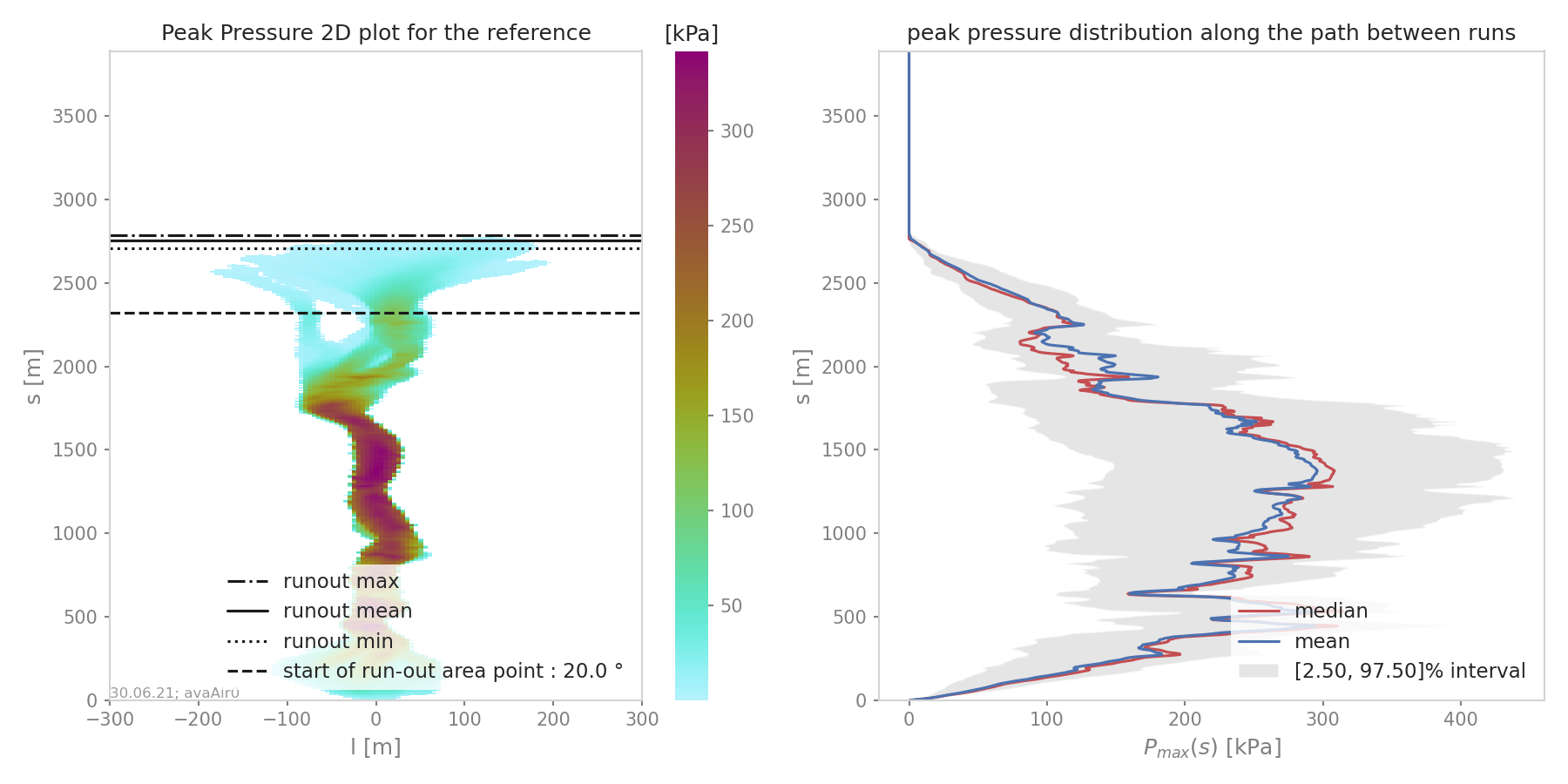
Fig. 18 Maximum peak pressure distribution along path

• “ROC” shows the normalized area difference between reference and other simulations.

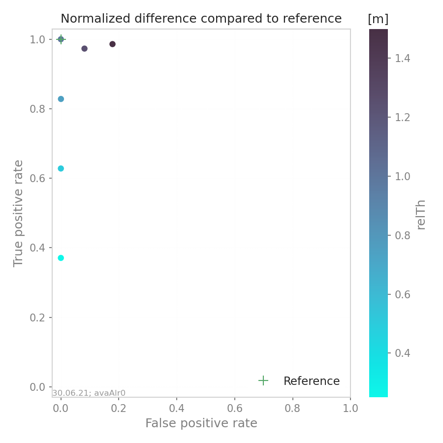
Fig. 19 Area analysis plot

• “relMaxPeakField” shows the relative difference in maximum peak value between reference and other simulation function of runout length

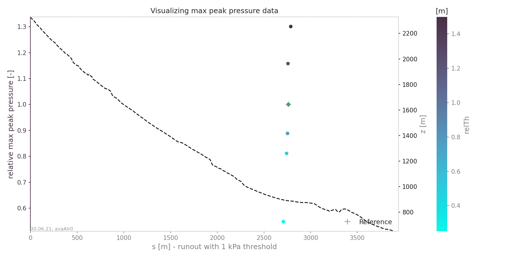
Fig. 20 Relative maximum peak pressure function of runout

The last plots “_i_ContourComparisonToReference” and “_i_AreaComparisonToReference” where “i” gives the number of the simulation plots the 2D difference with the reference and the statistics associated.

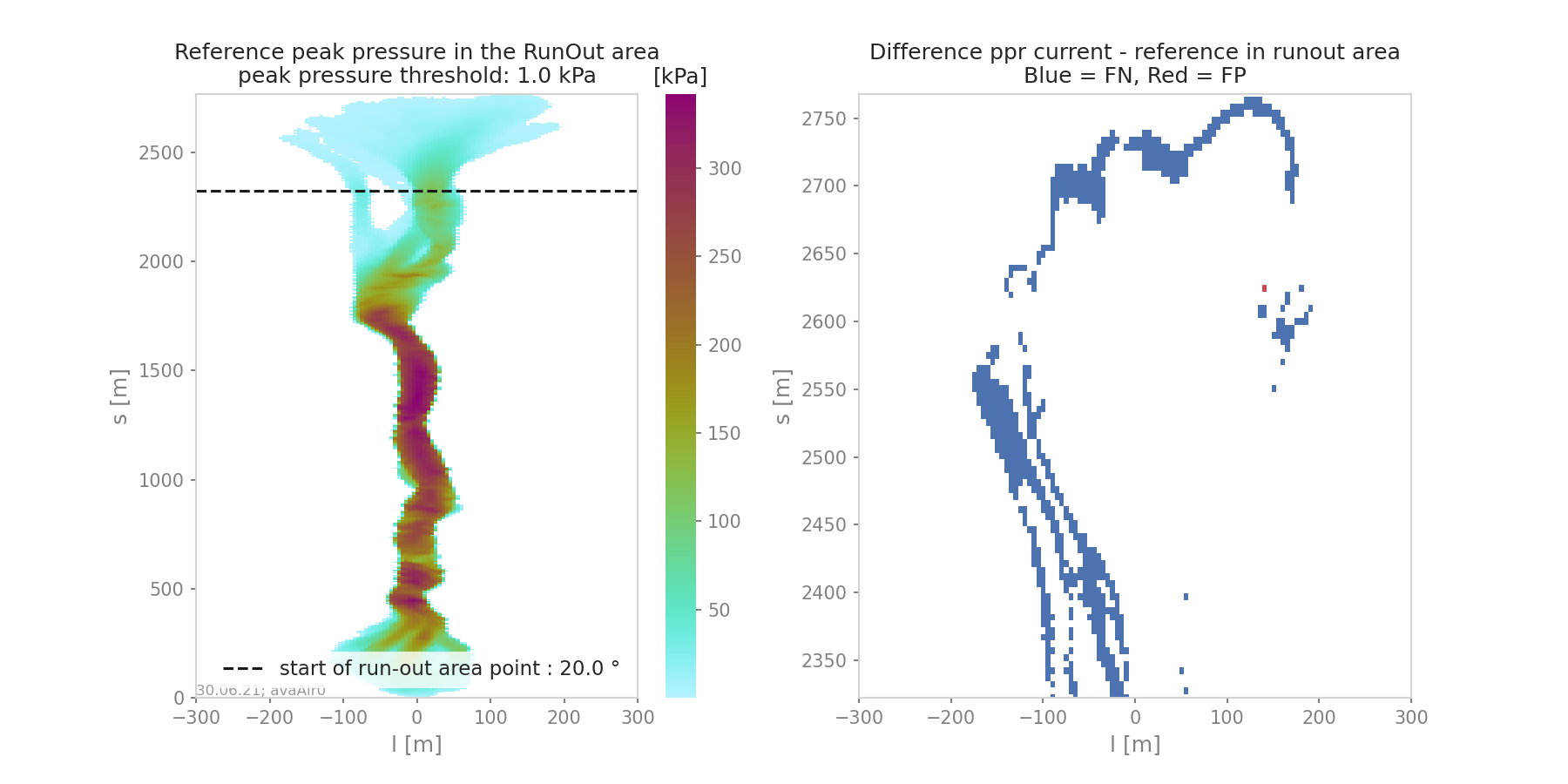
Fig. 21 Area comparison

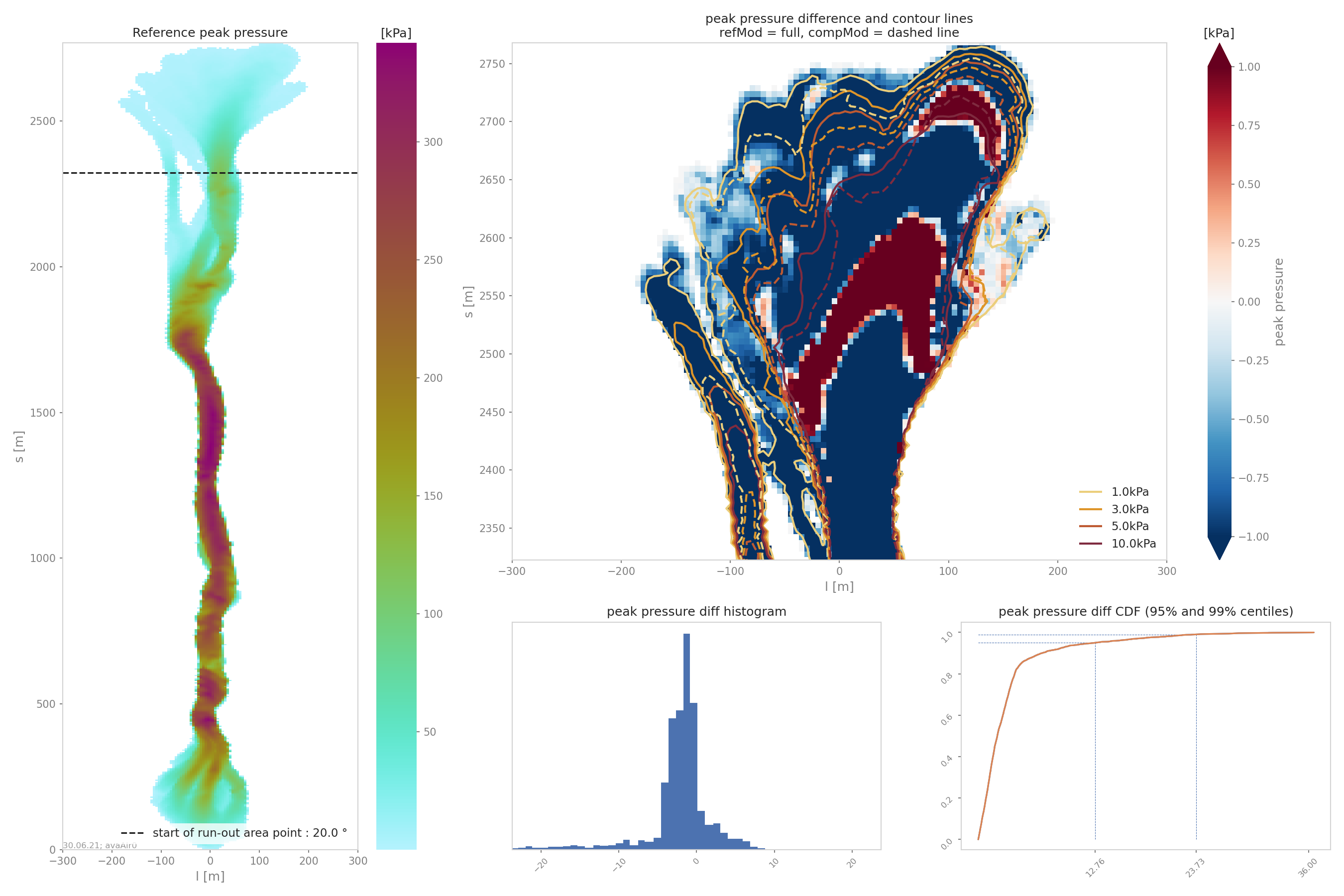
Fig. 22 Contour comparison

Configuration parameters

domainWidth

width of the domain around the avalanche path in [m]

startOfRunoutAngle

angle of the slope at the start of the runout zone [°]

resType

data result type for runout analysis

thresholdValue

limit value for evaluation of runout (according to the chosen resType)

contourLevels

contour levels for difference plot (according to the chosen resType)

diffLim

max/min of chosen resType displayed in difference plot

interpMethod

interpolation method used to project the a point on the input raster (chose between ‘nearest’ and ‘bilinear’)

distance

resampling distance. The given avalanche path is resampled with a 10m (default) step.

dsMin

float. Threshold distance [m]. When looking for the beta point make sure at least dsMin meters after the beta point also have an angle bellow 10° (dsMin=30m as default).

anaMod

computational module used to perform ava simulations

comModules

two computational modules used to perform ava simulations in order to compare the results

plotFigure

plot figures; default False

savePlot

Save figures; default True

WriteRes

Write result to file: default True